20.2.1 Short-Horizon Forecasts

20.2.1 Short-Horizon Forecasts

When the model parameters are known, the optimal forecast in (20.3) is

$$f_{T+h|T}=y_T+({\rho }^h-1)(y_T-{\varphi }^{\prime }{d}_T)+{\varphi }^{\prime }(d_{T+h}-d_T).$$

This results in an h-step-ahead forecast error of ${\sum }_{i=1}^h{\rho }^{h-i}{\epsilon }_{T+i}$ . The expected squared error loss is ${\sigma }_{\epsilon }^2(\bar{1}-{\rho }^{2h})/(1-{\rho }^2)$ which, as $T$ becomes large, converges to $h{\bar{\sigma }}_{\epsilon }^2;$ this result holds exactly if $\gamma =0$ . Hence the unpredictable component of y contributes a term that grows linearly in the forecast horizon. Local misspecification of the model retains this term and further adds a term that disappears at rate T .

Imposing a unit root is a common practice among forecasters. Under the assumption that $\rho =1$ , the forecast becomes $f_{T+h|T}=y_T+{\varphi }^{\prime }(d_{T+h}-d_T).\mathrm{If}{d}_t=1$ the second term is 0. If the model also contains a time trend, then ${\varphi }^{\prime }(d_{T+h}-d_T)=$ ${\varphi }_{2}h$ and the natural estimator for ${\varphi }_2$ is the mean of the change in $y_t-\mathrm{this}$ is the MLE under the misspecified model. We can study the costs and benefits of imposing a unit root by examining the asymptotic approximation to the forecast error $\begin{array}{r}{\sum }_{i=1}^h{\rho }^{h-i}{\epsilon }_{T+i}+({\rho }^h-1)(y_T-{\varphi }^{\prime }{d}_T)\end{array}$ for models where $\rho$ is local to 1. As just discussed, the first term is unpredictable and of higher order than the second component when $\rho$ is local to unity. These components contribute to the MSE but decline to 0 at rate T. To see this, note that

$$T^{1/2}({\rho }^h-1)(y_T-{\varphi }^{\prime }{d}_T)\Rightarrow -h\gamma {\sigma }_{\epsilon }M(1),$$

$$E[-h\gamma {\sigma }_{\epsilon }M(1){]}^2={\sigma }_{\epsilon }^2\left\{\frac{h^2\gamma ({\alpha }^2-1)e^{-2\gamma }}{2}+\frac{h^2\gamma }{2}\right\},\text{\hspace{1em}(20.5)}$$

where $M(1)$ is defined in (20.4). This second-order term is a function of how close $\rho$ is to 1 given the sample size (through $\gamma )$ , the forecast horizon $h,$ as well as the extent of the deterministic terms and the assumption on the initial condition. As expected, this term increases in both $\gamma$ (how far the root is from 1) and the forecast horizon— the effect of misspecification of the model compounds as h increases. In large enough samples the contribution of the initial condition is small and disappears quickly as γ moves away from 0 and so the second-order term is roughly equal to ${\sigma }_{\epsilon }^2{h}^2\gamma /2$ Equation (20.5) increases linearly in $\gamma$ and quadratically in $h,$ though note that the contribution of the unpredictable part of the forecast error increases linearly in $h.$ .

The expression in (20.5) can be used to understand the percentage increase in MSE from imposing $\rho =1$ . For reasonable values of ${\gamma }_{:}$ , the percentage increase in the MSE due to imposing a unit root rather than using the true value of $\rho$ is approximately equal to $h\gamma /(2T)$ . When $d_t$ includes a time trend there is an additional effect through the estimation of ${\varphi }_2$ . Using the mean of $y_{t+h}-y_t$ , the additional second-order term in the MSE can be approximated4 by ${\sigma }_{\epsilon }^2{h}^2(\gamma +2)/2$ This expression suggests that imposing the unit root on $\rho$ and estimating the coefficient on the time trend through the mean of the change in ${\gamma }_t$ increases the MSE5 by $h(\gamma +2)/(2T)$ . In either case, if the process is strongly mean reverting or the forecast horizon is long enough, imposing a unit root on the model will not yield good forecasts.

Rather than imposing a unit root, we could estimate the model parameters $(\rho ,\varphi )$ . Expressions under least squares estimation and serial correlation are available for this case in Phillips (1998). Ng and Vogelsang (2002) examine one-step-ahead forecast errors analytically for various OLS and GLS approaches and show that the asymptotic approximations to the first-order term (the term caused by estimation error) differ across estimation methods. Their simulation results suggest that GLS approaches (particularly ones incorporating the initial observation) outperform OLS approaches.

The third approach is to employ a pre-test for $\rho =1$ , imposing the unit root when the pre-test fails to reject, otherwise estimating the model parameters. Diebold and

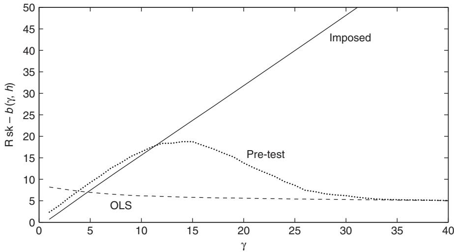
Figure 20.1: Short-horizon risk under three different approaches. The figure plots the risk component b as a function of the local-to-unity parameter $\gamma$ for three different approaches: (i) imposing a unit root (full line); (ii) estimating the model parameters (dash-dotted line); (iii) pre-testing for a unit root (dotted line). The figure assumes a short forecast horizon of $h=3$ periods and includes a constant deterministic term.

Kilian (2000) examine this approach in a Monte Carlo exercise and recommend pretesting for a unit root. As with all pre-test approaches (see chapter 6), the forecasting model based on a pre-test can itself be considered as an estimator and we can examine the resulting risk function. Elliott (2006) compares the risks for the three strategies of imposing a unit root, estimating the model parameters, and pre-testing using the Dickey and Fuller (1979) test for a unit root.

In each of these cases the risk for the AR(1) model is of the form ${\sigma }^2(1+$ $T^{-1}{b}_i(\gamma ,h))$ , where $i\in$ {impose unit root, estimate parameters by OLS, hybrid approach using a unit root pre-test}. The accompanying figures report the size of $b_i(\gamma ,h)$ as a function of $\gamma .$ The plots can be used to approximate the additional percentage MSE loss after dividing by the sample size. Figure 20.1 shows results for the model that only includes a constant, $d_t=1$ . The figure sets $h=3$ and shows results for various values of $\gamma .$ Figure 20.2 repeats this exercise when $d_t=(1,t)$ Some broad conclusions occur from these plots. First, imposing a unit root rather than estimating it works only very close to the region where the assumption of a unit root is true.6 Compared to estimating the autoregressive model, imposing a unit root is therefore likely to be a poor approach in practice. Second, as with all pre-testing methods, the risk function associated with using a unit root pre-test is attractive when the null of the pre-test is true or when the pre-test has power close to 1, i.e., for large values for $\gamma ,$ but the pre-test does poorly in an intermediate range where the power of the test is between the test size and 1. This is shown on the figures as a large hump in the risk function for intermediate values for $\gamma$

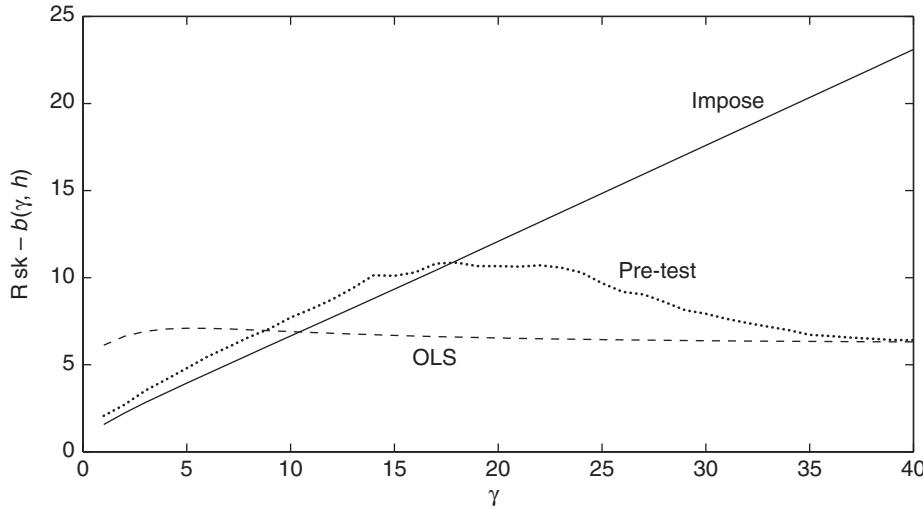
Figure 20.2: Short-horizon risk under three different approaches. The figure plots the risk component b as a function of the local-to-unity parameter γ for three different approaches: (i) imposing a unit root (full line); (ii) estimating the model parameters (dash-dotted line); (iii) pre-testing for a unit root (dotted line). The figure assumes a short forecast horizon of $h=3$ periods and includes a constant and a trend as deterministic terms.

These calculations all assume a persistent autoregressive process with a root close to 1. Other models can generate persistence in the data in a way that mimics unitroot-type dynamics. For example, breaks in the parameters of the process can look like permanent shocks, which result in unit root or near unit root behavior (Perron, 1989). Breaks are examined in chapter 19. Long memory models also have similar properties.