19.2 LIMITATIONS OF IN-SAMPLE TESTS FOR MODEL INSTABILITY

19.2 LIMITATIONS OF IN-SAMPLE TESTS FOR MODEL INSTABILITY

Once we allow the parameters of the model, ${\beta }_t$ , to change over time, there are many different ways to specify the precise way in which the parameters evolve. Parameters might shift from $\beta +d$ to $\beta$ just once at time $t=\tau$ as in Example 19.1.1 in which case the model for the parameters is ${\beta }_t=\beta +d1(t\le \tau )$ . Or, there could be multiple discrete shifts in the parameters:

$$\begin{array}{r}{\beta }_t=\{\begin{array}{ll}\beta +d_1& \mathrm{for}t\le {\tau }_1,\\ \beta +d_2& \mathrm{for}{\tau }_1<t\le {\tau }_2,\\ ⋮& ⋮\\ \beta +d_k& \mathrm{for}{\tau }_{k-1}<t\le {\tau }_k,\\ \beta & \mathrm{for}{\tau }_k<t.\end{array}\end{array}\text{\hspace{1em}(19.4)}$$

Rather than deterministic shifts in the parameters, we might consider a sequence of random perturbations,

$${\beta }_t={\beta }_{t-1}+{\epsilon }_t,\text{\hspace{1em}(19.5)}$$

also known as random walk breaks. If ${\epsilon }_t={\eta }_t{\tilde{\epsilon }}_t$ , where ${\eta }_t$ is a Bernoulli random variable and ${\tilde{\epsilon }}_t$ is drawn from a continuous distribution and is independent over time, the random walk breaks model is similar in form to the multiple discrete shifts model with an expected number of $pT$ breaks in the sample, where $\mathbf{p}$ is the probability parameter of the Bernoulli distribution. Mean reversion in the parameters can be captured by a specification of the form

$${\beta }_t=\kappa (\bar{\beta }-{\beta }_{t-1})+{\epsilon }_t,\text{\hspace{1em}(19.6)}$$

where $|\kappa |<1^{\prime }$ is the speed of mean reversion and $\hat{\beta }$ is the long-run mean for $\beta .$ An alternative to these models is that the coefficients follow a Markov switching process, oscillating between a finite number of states:

$${\beta }_t={\beta }_{s_t},s_t\in \{1,\dots ,K\},\text{\hspace{1em}(19.7)}$$

$$\mathrm{Pr}(s_t=i|s_{t-1}=j)=p_{ij}.$$

The existence of many different models for the break process, along with the lack of a uniformly most powerful test against any of these specific alternatives, has led to a large set of tests that attempt to distinguish the stable parameter model from models where the parameters break. For linear regression specifications with a single break, ad hoc tests based on least squares estimates of the break date have been employed (e.g., Andrews, 1993b), while families of optimal tests have been suggested by Andrews and Ploberger $(1994).$ Sequential methods for estimating the time of the break and testing for additional breaks in the remaining portions of the data have been suggested by Bai and Perron (1998) for a fixed number of breaks. For random walk breaks, Nyblom (1989) suggests a locally best test for more general sets of models and Elliott and Müller (2006) provide a point optimal test. Rossi (2005a) provides a test that is optimal with respect to a weighted average of power in a wellchosen direction.

For each of these break processes, tests for a fixed number of breaks have local power against models that converge to the stable no-break model at rate $T^{1/2}$ Assuming a single break, this means that $\delta =d\times \sec (\beta )$ , where $\mathsf{se}(\beta )$ is the standard deviation of the estimator for $\beta$ in the stable model. If we consider a break in the mean and Var $({\epsilon }_t)={\sigma }^2$ , this translates into a local break with magnitude $\delta =d\sigma T^{-1/2}$ . For the random walk model the variance of ${\epsilon }_t$ declines to 0 under the local alternative so $T\Delta {\beta }_t$ has a stable variance.

Important practical lessons emerge from the theoretical literature on break point testing and associated Monte Carlo studies. First, the power curves for optimal tests and many ad hoc tests are quite similar. This explains the continued use in practice of ad hoc tests for the single break model. Second, tests designed for one type of break process typically have power against other break processes. For example, tests for a single break often still reject under the alternative of random walk breaks. Elliott and Müller (2006) show that this conclusion extends to power equivalence between optimal tests; tests that are optimal for any member of a wide class of break processes have the same power against other break processes within this wide class. Rejections of a test for a particular break process therefore do not imply that the break process tested for is “correct”. Rather, it could be one of many processes. For sufficiently large values of either the break magnitude, $d,$ or the variance of $T\Delta {\beta }_t$ , break tests effectively have a power of 1 and so the presence of breaks of such magnitude is essentially known. For breaks of an order smaller than this, there is uncertainty over whether or not breaks really affected the parameters.

These features of break tests can be examined through Monte Carlo simulations. Figure 19.1 uses four Monte Carlo designs to examine the asymptotic power of tests for different types of breaks. In each case we consider breaks in the mean of an independent, normally distributed series. The upper left panel assumes that the break occurs at the center of the sample $(\tau =T/2);$ the upper right panel assumes two breaks, one at the 40th percentile of the sample, the other at the 60th percentile of the sample. Here δ is the sum of the magnitude of the two breaks. The lower panels assume that $T\Delta {\beta }_t$ is a random walk. In the lower left panel there is a 10% probability of a shock to $T\Delta {\beta }_t$ , while in the lower right panel a shock occurs every period. In both cases δ refers to the variance of the shocks normalized by the probability that the shock occurs.

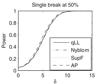
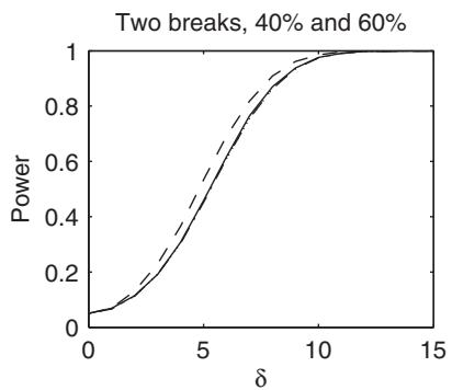
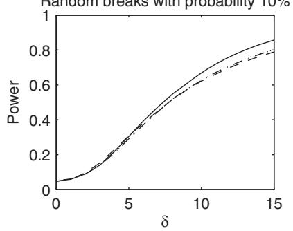
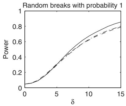
Figure 19.1: Solid line indicates qLL, dash-dot is Nyblom, dashes indicate the Andrews and Ploberger test, dots represent the SupF test power.

For each experiment figure 19.1 shows the asymptotic power for Andrews’ SupF test and the Andrews–Ploberger (AP) test—both designed to detect a single break— along with the power for the qLL test of Elliott and Müller (2006) and the Nyblom test for random walk breaks. The points noted above emerge clearly from these plots. First, the power curves are indeed similar and all tests have power against different types of break processes. As a consequence, rejection of a test designed to detect one particular break sequence is not evidence that the break sequence is in fact of this type. Rejections of the tests are clearly not suggestive of any specific form of instability—only of instability of some form.

As noted above, estimation results might suggest that some regressors should not be included in a forecasting model because their full-sample estimates are near 0 even though the regressors contain information useful to forecasting at time T. For models with a single break, an alternative strategy is to test jointly that $\beta ={\beta }_0$ and $\delta =0$ . This tests jointly that the value of the parameter in the forecasting model equals $0\left({\beta }_0=0\right)$ and the absence of a break $(\delta =0)$ . Hence, a test for whether $x_t$ is useful in forecasting $y_{t+h}$ in (19.1) that avoids failing to detect predictability due to an unknown break would involve testing both the parameter value $(\beta =0)$ and that there is no break $(\delta =0)$

Instead of jointly testing for a break and lack of predictability after the break (as in Rossi’s test if we set ${\beta }_0=0)$ , we could alternatively consider a hypothesis that tests the null of no predictability $(\beta =0)$ while controlling the test size regardless of the magnitude of δ. Elliott and Müller (2014) provide such a test when there is a break to a single element of $\nabla \cdot \nabla \beta .$ The test controls size asymptotically regardless of the size of the break, including no breaks.

Giacomini and Rossi (2009) look at the related question of whether forecast models estimated over one particular period are useful for forecasting future outcomes. Their test compares the in-sample and out-of-sample forecasting performance and seeks to predict forecast breakdowns as a means to predicting future breaks.