14.3 RISK FOR FORECAST COMBINATIONS

14.3 RISK FOR FORECAST COMBINATIONS

The majority of the combination methods suggested in the literature are to some extent ad hoc. A choice between forecast combination schemes, as with forecast methods in general, is really a choice of risk functions over data-generating processes deemed likely to be relevant for the particular problem at hand.

As in the analysis of the model selection methods in chapter 6, we can examine the risk for the different forecast combination procedures through Monte Carlo simulation. One problem that immediately presents itself is that most combination problems involve a large set of parameters, and the risk could depend on these parameters in a complicated fashion. Rather than attempt to be comprehensive, we employ a simple Monte Carlo design that is representative of the situations faced in practice and, more importantly, brings out some of the main practical issues. These are, first, that the Bates and Granger (1969) optimal forecast combination requires estimates of the m-dimensional combination weights and this added estimation error affects risk; second, equal-weighted forecast combinations often perform very well; and, third, no single combination method uniformly dominates for the same reasons as we discuss in chapter 6. In each Monte Carlo simulation there are 100 observations and for each model we report the average over 100,000 simulations.

Equal-weighted combination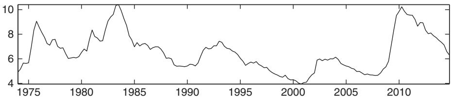

Previous best model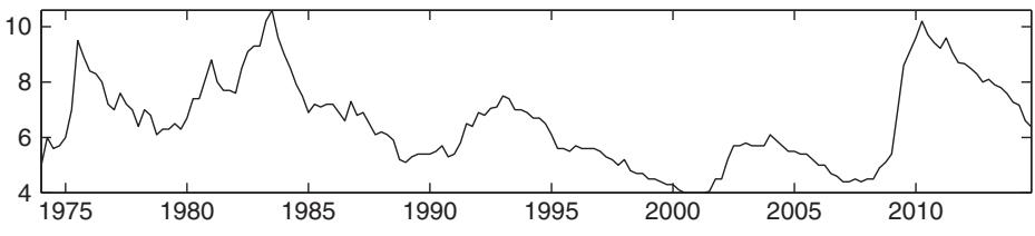

Inverse MSE weights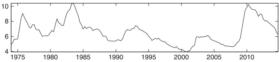

Figure 14.5: Combinations of the Survey of Professional Forecasters’ unemployment rate forecasts using the equal-weighted average (top), the previous best forecaster (middle), and inverse MSE weights (bottom). Ranking and estimation is based on a 5-year rolling window.

The design of the Monte Carlo is as follows. We assume that the forecast errors follow a normal distribution $e_{t+1|t}\sim \mathrm{N}(0,{\Sigma }_{\alpha })$ , where the variance–covariance matrix is such that each forecast has a variance of 1 and all forecasts are correlated with a correlation of 0.5 when $\alpha =0$ . Equal weights are optimal in the baseline case with when $\alpha =0$ . As α changes, the Bates–Granger optimal weights begin to spread out. The variance of the orthogonal and normally distributed residuals is chosen to be 1, which yields an $R^2$ for the regression of $y_{t+1}$ on the forecasts (without the restriction that the coefficients sum to 1) of about 40%; this value rises slightly with α.

Results from these simulations are shown in figure 14.7. The first column of panels shows results for $m=3$ forecasts while the second column assumes $m=10$ forecasts are being combined. The first row of the figure presents MSE values computed relative to the infeasible optimal MSE value which uses the population optimal weights. The second row plots the combination weights. The bottom row of panels shows the power of a test for equal weights (solid line) and the $R^2$ for the regression (dashed line).

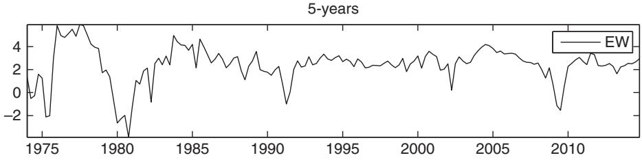
5-years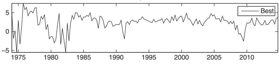

5-years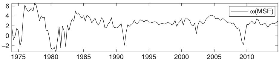

Figure 14.6: Combinations of the Survey of Professional Forecasters’ GDP growth rate forecasts using the equal-weighted average (top), the previous best forecaster (middle), and inverse MSE weights (bottom). Ranking and estimation is based on a 5-year rolling window.

The first row of graphs in figure 14.7 shows the mean squared error risk relative to the risk that would obtain with the infeasible optimal weights. For example, a value of 1.02 means a 2% higher risk than this benchmark. We examine four combination methods, namely, (a) optimal weights estimated by restricted least squares, as in equation (14.14); (b) equal weights, as in equation (14.12); (c) shrinking the estimate in (a) towards the estimate in (b) as in equation (14.16) with $g=0.5;$ and (d) weighting each estimator by the inverse of the estimated variance of the forecast error, adjusted so that the weights sum to 1, as in equation (14.18). As expected from the properties of least squares estimates, the risk for the restricted least squares combination method in (a) is flat across model designs; for $m=3$ the risk of this method is 1.02, while for $m=10$ the risk is 1.1. The risk for the combinations that use equal weights is also as expected. When the true weights are equal to each other $(\alpha =0)$ , this scheme obtains the optimal weights without estimation error. However, as the optimal weights become more disperse, the risk of the equal-weighted combination method increases due to the bias component of the MSE. Arguments that relate the better empirical performance of equal weights to the avoidance of estimation error rely on the weights being close enough to equal so that the bias component does not outweigh gains from reducing the variance component arising from not having to estimate the weights with data.

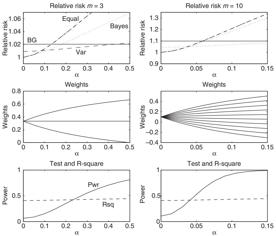
Figure 14.7: Risk for different combination schemes.

The panels in the second row in figure 14.7 show how the Bates–Granger optimal weights begin to spread out as we vary α along the horizontal axis.

As α rises the magnitude of a Wald test for equal weights increases to the point where the restriction would typically be rejected. This is illustrated in the third row of figure 14.7. It is noticeable that tests for equal weights need to reject with quite high power before the equal-weighted combination starts to produce higher risk than the combination schemes that rely on estimated weights. For m = 10 the weights must be far enough apart that the power of the test for equal weights is about 60%. For this case the optimal weights are quite disperse at this point. Shrinking the estimated weights towards the equal weights (combination scheme (c) in our simulations) has the expected effect, with risk typically falling between the risk of the two underlying methods that this shrinkage scheme is based on. However, the shrinkage combination method does not uniformly dominate either estimating the weights or imposing equal weights. Finally, ignoring correlations and using only the variances of the forecast errors (combination scheme (d)) does not result in a particularly attractive risk profile in these simulations.

When interpreting these results one should bear in mind that Monte Carlo studies reveal the risk at a few selected points in the parameter space, but often give a very incomplete picture of the trade-offs involved in choosing different combination schemes. Nevertheless, we think it is safe to conclude from these simulations that no combination method universally results in the lowest risk. Moreover, which method performs best will depend on the true data-generating process which of course is unknown. Hybrid methods that try to choose between using either estimated weights or equal weights do not uniformly dominate the underlying methods that they are based on.