14.2.4 Application to Survey Forecasts

14.2.4 Application to Survey Forecasts

We next illustrate some of the most popular combination methods in an empirical application that uses the type of survey data that are commonly used in forecasting.

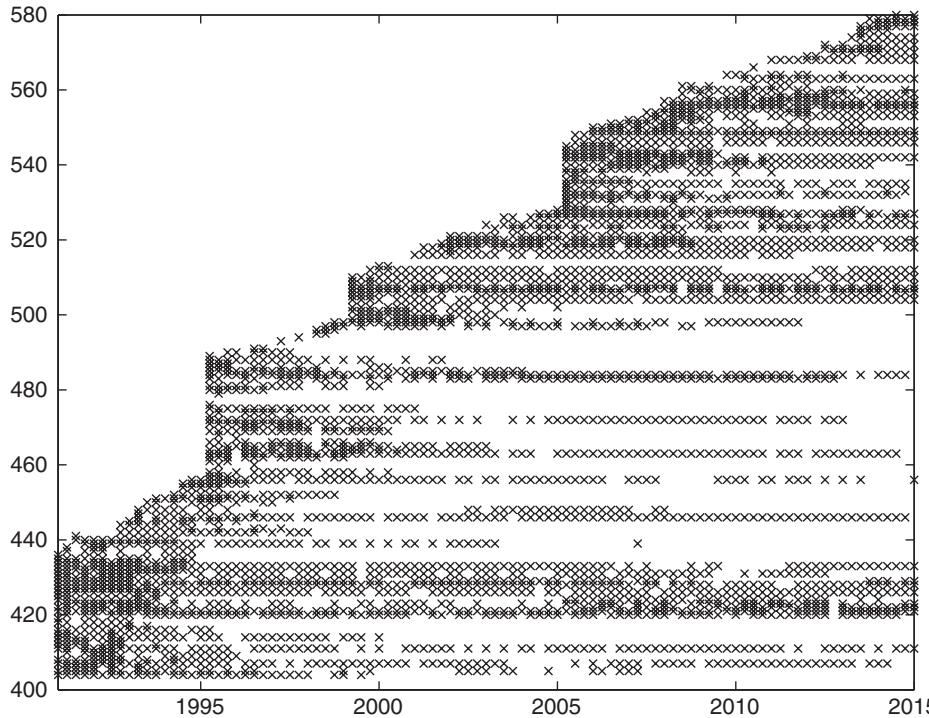
Figure 14.1: Reporting of GDP growth forecasts by participants with IDs above 400 in the Survey of Professional Forecasters. An “x” indicates that the survey participant reported a forecast for the following quarter, while an empty space indicates that the participant failed to report a prediction.

Primary sources of economic surveys used in macroeconomic forecasting include the Survey of Professional Forecasters and the Livingston Survey, both of which are maintained by the Federal Reserve Bank of Philadelphia, Blue Chip forecasts, Confederation of British Industry, Consensus Economics, and the University of Michigan survey of US consumers. In finance there is also the IBES data which survey analysts’ earnings forecasts, along with the Gallup investor survey, the Duke survey of CFOs, and the American Association of Individual Investors survey.

Surveys typically take the form of panels of relatively large numbers of participants’ forecasts. Importantly, the panels are unbalanced due to the frequent entry, exit, and reentry of individual participants.

As an empirical illustration, we consider one-quarter-ahead forecasts of the unemployment rate and growth in real GDP as reported by the Survey of Professional Forecasters. Forecasters includes commercial banks, individual experts, and professional forecasting firms and each forecaster is assigned a unique code that does not change over time. However, survey participants may exit and reenter the survey over time, and so forecast combination methods such as OLS estimation of the weights are not ideally suited for this type of unbalanced panel data.

Figure 14.1 illustrates how a subset of the individual forecasters (with IDs above 400) enter and exit the survey between 1991 and 2012. The majority of survey participants report real GDP growth forecasts for only relatively short periods of time, and even the forecasters with the longest track record experience some gaps in their reporting. The vertical trenches show when new groups of survey participants are added. Clearly the survey data constitute a highly unbalanced panel of forecasts.

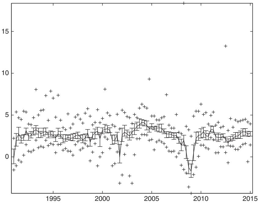
Figure 14.2: Median, interquartile range, highest and lowest point forecasts of real GDP growth from the Survey of Professional Forecasters. The middle of the box indicates the median forecast, outer bounds of the box show interquartile ranges, while the top and bottom “+” indicate the highest and lowest forecasts in a given quarter.

A purely statistical combination approach may miss out on any attrition bias that arises if forecasters exiting the survey—who do not subsequently reenter— exit because of poor forecasting performance. This behavior would resemble that observed among mutual funds which are more likely to close down if they have underperformed. If such attrition biases exist, forecast combinations might benefit from simply ignoring missing forecasts, unless they are randomly scattered in time.

Figure 14.2 shows the median, interquartile range, and highest and lowest point forecasts for real GDP growth over the period 1991Q2:2012Q4. There are considerable differences between the most pessimistic and optimistic forecasts in the sample. While movements in the median forecast are much smoother than those of the individual forecasts, there are some notable declines around 2002 and again in 2008 and 2009, coinciding with the recessions during those periods. These are also the main periods where the forecasts of GDP growth turned negative.

Figure 14.3 shows the identity of the best forecaster of the real GDP growth rate using MSE values estimated over the most recent 5-year (top) and 10-year (bottom) periods. A short evaluation window has the advantage that it can quickly identify skilled forecasters as well as quickly eliminate forecasters starting to produce poor forecasts. Conversely, the longer 10-year window can be used to obtain a more precise estimate of the individual forecasters’ average performance. In both cases there are periods with some forecasters dominating for a number of years, independently of whether a 5-year or a 10-year window is used. Note that some of this persistence in ranking is induced by the use of a rolling estimation window which is likely to lead to some persistence even in situations without persistence in skills.

5 Years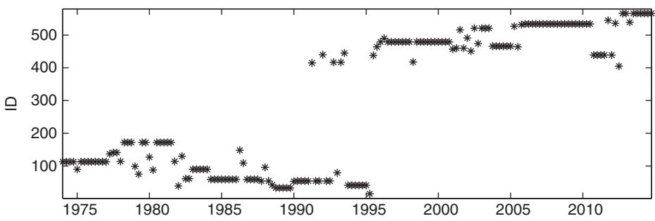

10 Years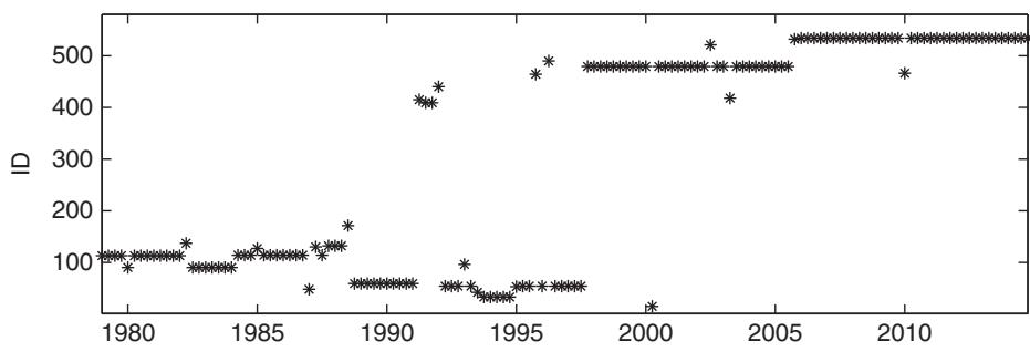

Figure 14.3: Identity of the participant in the Survey of Professional Forecasters with the best track record for GDP growth rate forecasts (measured by mean squared forecast error) over the previous 5 years (top) or the previous 10 years (bottom).

Figure 14.4 provides the same plot of the previous best forecast for the unemployment rate data. Again there is evidence that the identity of the best forecaster is persistent, but also that it shifts over time. Note that the shift from low IDs to higher IDs is related to sample attrition—survey participants with the lowest IDs drop out of the sample during the 1990s, whereas participants with the highest IDs are present only during the later parts of the sample after the sample gets replenished. However, even within the two blocks of participants there is a fair amount of turnover despite the fact that the rolling windows induce a certain amount of persistence in the rankings.

Figures 14.5 and 14.6 plot forecasts from the previous best forecaster, the equalweighted average computed across all survey participants that generate a forecast at a given point in time, and the inverse MSE-weighted average (14.18) for the unemployment rate (figure 14.5) and real GDP growth (figure 14.6). The inverse MSE weights and previous best forecaster variable use a 5-year rolling window.

5 Years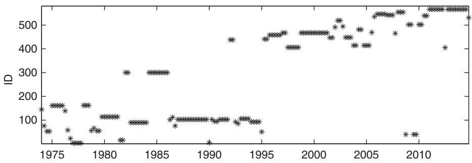

10 Years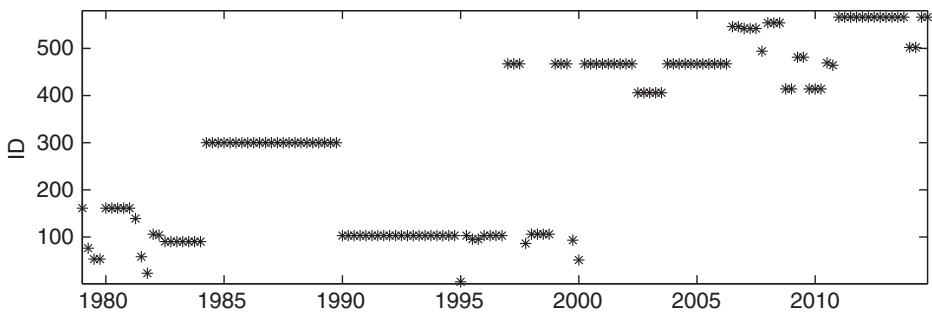

Figure 14.4: Identity of the participant in the Survey of Professional Forecasters with the best track record for unemployment rate forecasts (measured by mean squared forecast error) over the previous 5 years (top) or the previous 10 years (bottom).

For the unemployment series the long-run movements in the forecasts are very similar. This is to be expected given the highly persistent nature of this variable which means that a forecast based mainly on the current unemployment rate will capture most of the variation in this variable.

Conversely, we see bigger and quite pronounced differences in real GDP growth forecasts across the three approaches, suggesting that the choice of combination method is more important for this less persistent variable. Combining forecasts in proportion with the inverse of their MSE values leads to the most volatile forecasts for this variable.