13.5 INTERVAL AND QUANTILE FORECASTS

13.5 INTERVAL AND QUANTILE FORECASTS

Interval forecasts fall somewhere between density forecasts and point forecasts. They typically provide information about the most likely outcome as well as the degree of uncertainty surrounding a forecast as measured by the center and width of the interval forecast, respectively, assuming a symmetric distribution.

Example 13.5.1 (Conditional interval forecasts for Gaussian variable). For conditional location–scale models, $y_{t+1}={\mu }_{t+1|t}+{\sigma }_{t+1|t}{\eta }_{t+1},{\eta }_{t+1}\sim P_{\eta }(0,1)$ a typical interval forecast is that the outcome $y_{t+1}$ falls in the interval $[p_{t+1|t}^1(\alpha ),p_{t+1|t}^{\mathrm{u}}(\alpha )]$ for some probability $1-\alpha ,\alpha \in (0,1/2)$ , where

$$\begin{array}{rl}& p_{t+1|t}^1={\mu }_{t+1|t}+{\sigma }_{t+1|t}{P}_{\eta }^{-1}(\alpha /2),\\ & p_{t+1|t}^{\mathrm{u}}={\mu }_{t+1|t}+{\sigma }_{t+1|t}{P}_{\eta }^{-1}(1-\alpha /2).\end{array}\text{\hspace{1em}(13.43)}$$

If $P_{\eta }$ is Gaussian and $\alpha =0.05$ , this simplifies to

$$\begin{array}{rl}& {\mathbf{p}}_{t+1\mid t}^1={\mathbf{\mu }}_{t+1\mid t}-1.96{\mathbf{\sigma }}_{t+1\mid t},\\ & {\mathbf{p}}_{t+1\mid t}^{\mathrm{u}}={\mathbf{\mu }}_{t+1\mid t}+1.96{\mathbf{\sigma }}_{t+1\mid t}.\end{array}$$

Example 13.5.2 (Interval forecasts using a two-piece normal distribution). If the density follows the two-piece normal distribution in (13.29) with mean ${\mu }_{t+1|t}$ and variances below and above the mean of ${\cdot }_{{\sigma }_1^2,{\sigma }_2^2}$ , respectively, the α quantiles $q_{\alpha }$ are

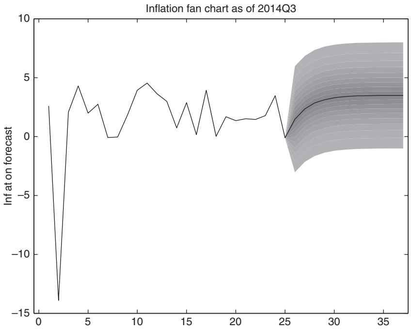
Figure 13.9: Fan charts generated by the two-piece exponential density, showing the predicted median and the 75% and 90% ranges for the predictive density.

given by

$$q_{\alpha }=\{\begin{array}{ll}{\mu }_{t+1\mid t}+{\sigma }_1{\Phi }^{-1}\left(\frac{\alpha }{C\sqrt{2\pi }{\sigma }_1}\right)& \mathrm{for}\alpha \le \frac{{\sigma }_1}{{\sigma }_1+{\sigma }_2},\\ {\mu }_{t+1\mid t}+{\sigma }_2{\Phi }^{-1}\left(\frac{\alpha +C\sqrt{2\pi }{\sigma }_2-1}{C\sqrt{2\pi }{\sigma }_2}\right)& \mathrm{for}\alpha >\frac{{\sigma }_1}{{\sigma }_1+{\sigma }_2},\end{array}$$

where $C=\sqrt{2/\pi }({\sigma }_1+{\sigma }_2{)}^{-1}$ ; see Banerjee and Das (2011).

Figure 13.9 plots a fan chart for quarterly inflation as of 2014Q3, using a two-piece exponential distribution fitted to quarterly inflation data. The solid line tracks the actual inflation rate during the six years leading up to 2014Q3 (observation 24) and tracks the point forecast for the subsequent three years (12 quarters). The different shades indicate 5% probability ranges for future inflation. While the point forecast for inflation is quite smooth, it is surrounded by considerable uncertainty, particularly at horizons greater than one year.

To construct interval forecasts for location–scale models, three estimates are required, namely an estimate of the conditional mean, ${\mu }_{t+1|t:}$ , an estimate of the conditional volatility, ${\sigma }_{t+1|t}$ , and an estimate of the distribution function of the normalized innovation, $P_{\eta },$ so that $P_{\eta }^{-1}(\alpha /2)$ and $P_{\eta }^{-1}(1-\alpha /2)$ can be evaluated. Here $P_{\eta }^{-1}$ is the quantile function. Hansen (2006) discusses ways to allow for parameter estimation uncertainty in the construction of interval forecasts.

Many parametric density forecast models lead to quantile forecasts that are simple to derive. For example, conditional location–scale models with Gaussian innovations

imply quantiles of the form

$$q_{\alpha }(y_{t+1}|z_t)={\mu }_{t+1|t}+{\sigma }_{t+1|t}{P}_{\mathrm{N}}^{-1}(\alpha ),\alpha \in (0,1),\text{\hspace{1em}(13.44)}$$

where $P_{\mathrm{N}}$ is the standard normal distribution function and $P_{\mathrm{N}}^{-1}$ is the associated quantile function.

An alternative to this procedure is to separately model individual quantiles. This approach has gained interest particularly in value at risk (VaR) calculations in finance. Under the recommendations of the Basel committee, VaR estimates should be reported by banks as part of their risk management practices. VaR estimates are essentially left-tail quantile forecasts and so require banks to have ways to predict the quantiles for their asset values.

Predictability in individual quantiles can be captured in different ways by modeling $q_{\alpha }(y_{t+1}|Z_t)$ , the conditional quantile for $y_{t+1}$ given current information, $Z_t$ Since the full conditional distribution function does not need to be specified, such regressions are semiparametric. Typically the conditional quantile $q_{\alpha }(y_{t+1}|Z_t,\beta )$ is specified up to some unknown finite-dimensional parameter vector, $\beta .$ Given an estimate, $\hat{\mathbf{\beta }},$ quantile forecasts can be computed as $q_{\alpha }(y_{t+1}|Z_t,\hat{\beta })$ . For example, a linear quantile model would take the form

$$q_{\alpha }(y_{t+1}|Z_t,\beta )={\beta }_{0\alpha }+{\beta }_{1\alpha }{z}_t.\text{\hspace{1em}(13.45)}$$

Since the slope coefficient $({\beta }_{1\alpha })$ can differ across quantiles, this model is quite flexible and nests existing models from the literature, including the benchmark model ${\beta }_{1\alpha }=$ 0 that assumes a constant distribution.

Generalizations of the quantile model that admit autoregressive dynamics have been proposed by Engle and Manganelli (2004). The so-called CAViaR models include last period’s conditional quantile and the absolute value of last period’s realization, $|y_t|.$ , as predictor variables. For example, the symmetric absolute value and asymmetric slope models of Engle and Manganelli take the form

$$\begin{array}{rl}& q_{\alpha }(y_{t+1}|Z_t)={\beta }_{0\alpha }+{\beta }_{1\alpha }{q}_{\alpha }(y_t|Z_{t-1})+{\beta }_{2\alpha }|y_t|,\\ & q_{\alpha }(y_{t+1}|Z_t)={\beta }_{0\alpha }+{\beta }_{1\alpha }{q}_{\alpha }(y_t|Z_{t-1})+{\beta }_{2\alpha }\max (0,y_t)+{\beta }_{3\alpha }\min (0,y_t),\end{array}\text{\hspace{1em}(13.46)}$$

where $q_{\alpha }(y_t|z_{t-1})$ is the lagged α-quantile. If ${\beta }_{1\alpha }>0$ , this specification is consistent with persistence in the α-quantile for the predicted variable. Notice that it is important to let the coefficients depend on α. For example, the tail dynamics observed in many financial time series tend to be highly persistent and can be captured by letting α be close to either 0 (left tail) or 1 (right tail). Conversely, for such series it is often found that there is little persistence in the conditional distribution of the center of the distribution as captured by the median (α = 0.5).