13.2.3 Refinements to GARCH Models

13.2.3 Refinements to GARCH Models

Numerous refinements to (13.7) that account for asymmetric effects of positive and negative volatility shocks have been proposed in the literature. For example, the threshold GARCH model allows negative and positive shocks to have different impact on future volatility:

$${\sigma }_{t+1|t}^2=\omega +{\alpha }_1{\epsilon }_t^2+\lambda {\epsilon }_t^{2}1\left({\epsilon }_t<0\right)+{\beta }_1{\sigma }_{t|t-1}^2,\text{\hspace{1em}(13.13)}$$

where 1(·) is an indicator function that equals 1 if the condition in the bracket holds, and otherwise is 0. Here the additional news effect of negative shocks on the conditional variance is λ. In empirical work it is frequently found that λ is positive, as negative shocks affect the conditional volatility more strongly than positive shocks. This is sometimes labeled the leverage effect.3 Forecasting volatility with (13.13) requires predicting the probability of positive versus negative shocks whenever these affect future volatility differently. Under the assumption that negative and positive shocks are equally likely, i.e., $\mathrm{Pr}({\eta }_t<0)=\mathrm{Pr}({\epsilon }_t<0)=0.5$ , it follows from (13.13) that

$$\begin{array}{rl}& {\sigma }_{t+1\mid t}^2=\omega +({\alpha }_1+0.5\lambda ){\epsilon }_t^2+\lambda {\epsilon }_t^2[1\left({\epsilon }_t<0\right)-0.5]+{\beta }_1{\sigma }_{t\mid t-1}^2\\ & ={\sigma }^2+({\alpha }_1+0.5\lambda +{\beta }_1)\left[{\sigma }_{t\mid t-1}^2-{\sigma }^2\right]\\ & +({\alpha }_1+0.5\lambda ){\sigma }_{t\mid t-1}^2[{\eta }_t^2-1]+\lambda {\epsilon }_t^2[1\left({\epsilon }_t<0\right)-0.5],\end{array}\text{\hspace{1em}(13.14)}$$

where now ${\sigma }^2=\omega (1-{\alpha }_1-0.5\lambda -{\beta }_1{)}^{-1}$ . Using that $E_t[{\eta }_{t+i}^2-1]=0$ and $E_t[1({\epsilon }_{t+i}<0)-0.5]=0$ for $i\ge 1$ , we get the h-step-ahead forecast of the one-period conditional variance as (see Andersen et al., 2006)

$${\sigma }_{t+h\mid t}^2={\sigma }^2+({\alpha }_1+0.5\lambda +{\beta }_1{)}^{h-1}\left({\sigma }_{t+1\mid t}^2-{\sigma }^2\right).\text{\hspace{1em}(13.15)}$$

Compared with the earlier formula for multistep forecasts from the GARCH(1,1) model (13.11), multistep forecasts from the threshold GARCH model in (13.15) are anchored on a different mean value and also can have different persistence, i.e., ${\alpha }_1+0.5\lambda +{\beta }_1$ versus ${\alpha }_1+{\beta }_1$ , although it should be noted that the estimates of ${\alpha }_1$ and ${\beta }_1$ in the two models are likely to be different due to the inclusion of the asymmetry term.

Since the conditional variance cannot be negative, models for the conditional variance must impose nonnegativity of the variance. This is usually not a concern in practice for specifications such as the GARCH(1,1) model since volatility is often highly persistent and ω, ${\alpha }_1.$ , and ${\beta }_1$ are all clearly positive. Another concern may be that the conditional variance is close to following an integrated process with ${\alpha }_1+{\beta }_1$ close to 1.

One way to deal with the nonnegativity constraint on the conditional variance is to instead model the logarithm of volatility which is not subject to such concerns. This gives rise to the EGARCH model of Nelson (1991):

$$\log ({\sigma }_{t+1|t}^2)=\omega +{\alpha }_1(|{\eta }_t|-E\left[|{\eta }_t|\right])+{\beta }_1\log ({\sigma }_{t|t-1}^2)+\lambda {\eta }_t.\text{\hspace{1em}(13.16)}$$

Again this model allows for asymmetric news effects of positive and negative shocks: positive shocks $({\eta }_t>0)$ impact the log conditional variance by $\lambda +{\alpha }_1.$ , while the effect of negative shocks is $\lambda -{\alpha }_1$

An important advantage of the EGARCH specification is that there is no need to impose constraints on the parameters to ensure that the conditional volatility remains nonnegative. Conversely, a disadvantage of (13.16) is that while it easily delivers conditional forecasts of the h-step log-variance, log $({\sigma }_{t+h|t}^2)$ , typically the object of interest is not to predict the logarithm of the variance, but rather the variance itself, ${\sigma }_{t+h|t}^2$ . There are no analytical expressions for ${\sigma }_{t+h|t}^2$ under the EGARCH model. Instead Monte Carlo simulation of the sequence of one-step density forecasts can be used to generate multistep volatility forecasts. This requires using numerical methods and so is a bit more involved.4

GARCH-type models can easily be generalized to allow for predictability from other state variables, $z_t,$ , or to let the volatility forecast affect the forecast of the conditional mean. For example, Glosten et al. (1993) consider an EGARCH-type model for the trade-off between risk and returns on stocks:

$$\begin{array}{c}{y}_{t+1}={\mu }_0+{\mu }_1{\sigma }_{t+1\mid t}+{\epsilon }_{t+1},{\epsilon }_{t+1}\sim \mathrm{N}(0,{\sigma }_{t+1\mid t}^2),\\ \log ({\sigma }_{t+1\mid t}^2)={\omega }_0+{\beta }_1\log ({\sigma }_{t\mid t-1}^2)+{\delta }_1\left|\frac{{\epsilon }_t}{{\sigma }_{t\mid t-1}}\right|+{\delta }_2\frac{{\epsilon }_t}{{\sigma }_{t\mid t-1}}+{\delta }_3{z}_t.\end{array}\text{\hspace{1em}(13.17)}$$

In this model the log conditional variance, ${\sigma }_{t+1|t}^2,$ depends on the state variable, $z_t,$ the lagged conditional variance, ${\sigma }_{t\mid t-1}^2.$ as well as current innovations, ${\epsilon }_t,$ whose effect may depend on whether the shocks are positive or negative. Moreover, the conditional mean is affected by the conditional volatility forecast—a phenomenon often labeled the ARCH-in-mean effect. This is consistent with the notion that investors expect higher returns, the higher the predicted volatility.

A property of the volatility models described so far is that the effect on future average volatility of a shock decays very fast, i.e., at an exponential rate as can be seen from formulas such as (13.11) and (13.15). Empirical studies of absolute or squared security returns sometimes find that their autocorrelations decay at a slower hyperbolic rate rather than at an exponential rate, suggesting that there is long memory in the volatility process.5 To capture this, Baillie, Bollerslev, and Mikkelsen (1996) propose a so-called fractionally integrated, FIGARCH(1,d,1) process for the conditional variance:

$${\sigma }_{t+1|t}^2=\omega +{\beta }_1{\sigma }_{t|t-1}^2+[(1-{\beta }_{1}L-(1-{\alpha }_{1}L-{\beta }_{1}L))(1-L{)}^d]{\epsilon }_t^2.$$

Slow decay in autocorrelations of the variance occurs if $0<d<1$ . These authors also show that variance forecasts can be generated recursively using a chain rule of the form

$${\sigma }_{t+h|t+h-1}^2=\frac{\omega }{1-{\beta }_1}+\lambda (L){\sigma }_{t+h-1|t+h-2}^2,h>0,$$

where the coefficients of the polynomial $\lambda (L)=1-(1-{\beta }_{1}L{)}^{-1}(1-{\alpha }_{1}L-$ ${\beta }_{1}L)(1-L{)}^d$ are generated recursively:6

$$\begin{array}{rl}& {\lambda }_1={\alpha }_1+d,\\ & {\lambda }_j={\beta }_1{\lambda }_{j-1}+[(j-1-d)j^{-1}-({\alpha }_1+{\beta }_1)]{\delta }_{j-1},j\ge 2,\\ & {\delta }_j={\delta }_{j-1}(j-1-d)j^{-1}.\end{array}$$

For many GARCH models the multistep predictive density is not obtainable in closed form. In such cases, numerical methods can be used to generate multistep volatility forecasts. As explained by Andersen et al. (2006), such forecasts can be computed by using the convolution of the one-step conditional distributions which are typically fully specified by the GARCH models:

Parameter estimates for GARCH(1,1) and GJR(1,1) models fitted to daily stock returns on the S&P500 index.

$$\begin{array}{rl}& p_Y(y_{t+h}|Z_t)=\int \int \cdots \int p_Y(y_{t+h}|z_{t+h-1})p_Y(y_{t+h-1}|z_{t+h-2})\cdot \cdot \cdot P\mathbf{Y}(y_{t+1}|Z_t)\\ & \times d{y}_{t+h-1}\dots d{y}_{t+1}.\end{array}$$

The procedure is to draw normalized residuals, ${\eta }_{t+1}^b,\dots ,{\eta }_{t+h}^b$ , and then recursively generate values of the conditional volatility, ${\sigma }_{t+h+1|t+h}^b,$ using the preferred GARCH model, g :

$$\begin{array}{rl}& y_{t+j+1}^b=\mu +{\sigma }_{t+j+1|t+j}^b{\eta }_{t+j+1}^b,\\ & {\sigma }_{t+j+1|t+j}^b=g\left(\{{\sigma }_{t+i|t+i-1}^b,{\eta }_{t+i}^b{\}}_{i=1}^j;\theta \right).\end{array}$$

This generates a simple Monte Carlo estimate of the predictive density $p_Y(y_{t+h}|Z_t)$ For example, an estimate of the h-step-ahead conditional variance given current information, ${\sigma }_{t+h+1|t}^2,$ can be obtained by iterating on the above equations and averaging across Monte Carlo simulations,

$${\hat{\sigma }}_{t+h+1|t}^2=\frac{1}{B}\sum _{b=1}^B{\left({\sigma }_{t+h+1|t}^b\right)}^2,b=1,\dots ,B.$$

In the simplest case, ${\eta }_{t+i}^b$ is drawn from a normal distribution. However, since the innovations need not be Gaussian, another possibility is to use estimated, standardized residuals, ${\hat{\eta }}_t=(y_t-{\hat{\mu }}_{t|t-1})/{\hat{\sigma }}_{t|t-1}$ to construct the c.d.f. for the residuals, ${\hat{P}}_{\eta },$ and then draw with replacement from this distribution. This can help capture features of the normalized residuals such as skews and fat tails.

Empirical estimates for GARCH models applied to many security returns suggest a high degree of persistence in the conditional variance. As an example, we estimated GARCH(1,1) and GJR models (described in equations (13.8) and (13.17)) for daily stock returns on the S&P500 index over the period 1990:01:01–2015:03:31. The resulting parameter estimates are reported in table 13.1. The volatility process is highly persistent, with GARCH(1,1) estimates of ${\hat{\alpha }}_1=0.110$ ${\hat{\mathbf{\beta }}}_1=0.877$ , so their sum (0.987) is close to unity. Figure 13.1 shows a plot of the associated (in-sample) conditional one-step-ahead volatility forecasts. Periods of low volatility around 2005 and, later, after 2012, are interspersed with periods of extremely high volatility such as during the fall of 2008. The GARCH(1,1) and GJR(1,1) estimates share common trends and are broadly similar.

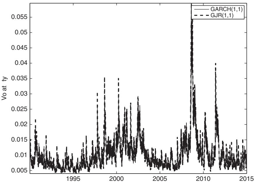
Figure 13.1: One-step-ahead conditional volatility forecasts generated by GARCH(1,1) and GJR models fitted to daily stock market returns.

Figure 13.2 plots the conditional volatility estimates implied by the GARCH(1,1) and GJR models during a few months in 2014. Focusing on this shorter sample allows us to better highlight the differences between the volatility estimates implied by these two models. Differences are largest following days with large negative shocks to returns because these have a larger effect on the GJR volatility forecast than on the forecast implied by the GARCH(1,1) model.