12.1 POINT AND DENSITY FORECASTS FOR BINARY OUTCOMES

12.1 POINT AND DENSITY FORECASTS FOR BINARY OUTCOMES

We first introduce some notation needed in the analysis. Let $Y=1$ if some event occurs, while $Y=0$ if the event does not occur, and let the random variable $p(Z)$ denote the probability that $Y=1$ given Z. The choice of how we map the two outcomes to specific numbers is arbitrary, some methods in the literature use the normalization that the outcome equals −1 when the event does not occur. To cover this case we also define $\tilde{Y}=2Y-1$ which transforms the outcome space to {−1, 1}. The literature on binary forecasting uses both of these codings; either leads to the same results, although some of the expressions change. We focus on $Y,$ but also provide some results for $\tilde{Y}$ to map back to the original papers.

Typically the conditional mean $E\left[Y|Z=z\right]$ provides a point forecast for the outcomes of $Y$ whereas $P\left[Y|Z=z\right]$ gives the density forecast. For binary outcomes, however, this is not the case. Since Y takes one of only two values, then $E\left[Y|Z=z\right]=$ $P\left[Y|Z=z\right]$ and so estimating one is the same as estimating the other. Point forecasts on the other hand should have the same support as the outcome, so point forecasts for forecasting Y should be either 0 or 1. This will never be the conditional mean for the Bernoulli distribution except in trivial cases where all outcomes are identical or the outcome is known with certainty, i.e., we have $E\left[Y|Z=z\right]=P\left[Y=1|Z=z\right]$ ， and hence $0<E\left[Y=1|Z=z\right]=P\left[Y=1|Z=z\right]<1$ , excluding trivial cases.

A density forecast along with a utility function can be used to generate a point forecast, so the standard relation between these two objects holds despite the different relations they individually bear with the conditional expectation. As usual, we are interested in predicting the outcome with a forecast function $f(Z)$ . The utility function of the decision maker, $U(f,Y,Z)$ , depends on the action, $f;$ the outcome, $Y;$ and potentially all or some subset of the covariates, Z. If the forecast and outcome are both binary, utility can take only four possible values $U_{f,y}$ for any z:

$$U(f,y,z)=\{\begin{array}{ll}{u}_{1,1}(z)& \mathrm{if}f=1\mathrm{and}y=1,\\ u_{1,0}(z)& \mathrm{if}f=1\mathrm{and}y=0,\\ u_{0,1}(z)& \mathrm{if}f=0\mathrm{and}y=1,\\ u_{0,0}(z)& \mathrm{if}f=0\mathrm{and}y=0.\end{array}\text{\hspace{1em}(12.1)}$$

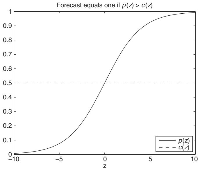
Figure 12.1: Probability forecast versus cutoff.

Sensible loss functions satisfy that $u_{1,1}(z)>u_{0,1}(z)$ and $u_{0,0}(z)>u_{1,0}(z)$ for all $z$ so that a correct forecast is always superior to an incorrect one. The utility from correctly predicting a negative outcome need not be equal to the utility from correctly predicting a positive outcome, so we could have $u_{1,1}(z)\ne u_{0,0}(z)$ . For example, if the predicted outcome is whether a stock price goes up $(y=1)$ or down $(y=0)$ , we would have $u_{1,1}(z)<u_{0,0}(z)$ if being correct when the market falls is better than being correct when it rises. This simply says that avoiding losses is better for investors than making gains and might reflect a concave utility function.

Recalling from chapter 3 that risk can be defined as the negative of expected utility, $R(\theta ,f,Z)=E\left[-U(f(Z),Y,Z)\right]$ , a simple result lets us characterize the optimal density forecast with binary outcomes. Conditioning on $Z,$ the risk is minimized by setting $f(Z)=1$ , i.e., forecasting a positive outcome, when

$$p(Z)>c(Z)\equiv \frac{u_{0,0}(Z)-u_{1,0}(Z)}{u_{1,1}(Z)-u_{0,1}(Z)+u_{0,0}(Z)-u_{1,0}(Z)}.\text{\hspace{1em}(12.2)}$$

We refer to $c(Z)$ as the cutoff point at which the forecast switches between its two possible outcomes. When the probability that $Y=1$ is greater than some cutoff, $c(Z)$ , determined by the utility function, the optimal forecast is $f(Z)=1$

A common choice of cutoff is $c(Z)=\mathrm{0.5.}$ . This choice is illustrated in figure 12.1, which shows for a univariate Z the situation where $p(Z)$ is monotonically increasing in Z with $c(Z)=0.5$ . The model forecasts an outcome of $\mathbf{y}=1$ for $p(z)>c(z)$ . This choice is optimal when $u_{0,0}(Z)-u_{1,0}(Z)=u_{1,1}(Z)-u_{0,1}(Z)$ , i.e., when the relative utilities from a correct forecast versus an incorrect one are equal2 regardless of the direction of Y. Choices of cutoff other than 0.5 are relevant in situations where these marginal gains differ. For example, if the gain for $y=1$ is bigger than that for $y=0$ we could set the cutoff below 0.5 so as to “overweight” the more valuable forecasts, $f=1$

When the utility function does not depend on $Z,c(Z)=c$ , and the utility- maximization problem can be reduced through a variety of renormalizations. Without loss of generality, we can subtract $u_{1,1}$ from the utility for $y=1$ , so that the utility equals 0 for a correct positive forecast, while for a false negative it is equal to ${\tilde{u}}_{0,1}=u_{0,1}-u_{1,1}<0$ . Similarly, for $y=0$ we can subtract $u_{0,0}$ from utility, thereby setting the utility for a correct negative forecast to 0 and ${\tilde{u}}_{1,0}=u_{1,0}-u_{0,0}<0$ for a false positive. This change leaves the numerator and denominator of c in (12.2) unchanged and allows us to write

$$c\equiv \frac{{\tilde{u}}_{1,0}}{{\tilde{u}}_{0,1}+{\tilde{u}}_{1,0}}.$$

In this case we can use that utility has no natural units to normalize ${\tilde{u}}_{1,0}+{\tilde{u}}_{0,1}=-1$ This leaves us with $c=-{\tilde{u}}_{1,0},{\tilde{u}}_{0,1}=-(1-c)$ , and the simplified representation3

$$U(f,y,c)=\{\begin{array}{ll}0& \mathrm{if}f=1\mathrm{and}y=1,\\ -c& \mathrm{if}f=1\mathrm{and}y=0,\\ -(1-c)& \mathrm{if}f=0\mathrm{and}y=1,\\ 0& \mathrm{if}f=0\mathrm{and}y=0,\end{array}$$

where $c>0$ and the utility function is expressed directly as a function of the cutoff value, c .

If we construct distributional forecasts of the outcome $p(Z)$ , we must employ a utility function on the probability for both estimation and forecast evaluation purposes. One probability forecast $p(Z)$ is better than another if it results in a higher utility for all possible cutoffs, c , i.e., $p(Z)$ is the dominant rule regardless of the utility function. If $p(Z)$ were known, this would be the dominant rule. More likely, however, $p(Z)$ has to be estimated and the model is misspecified and so $p(Z)$ is not equal to the true conditional probability. In this situation, some models could be best for certain regions of $c,$ while other models could be best for other regions of c.

The scoring rule used for estimating a loss function, if proper, can be related directly to a weighting function over the possible cutoffs, c, which range from 0 to 1.

Proper scoring rules take the form

$$L(p,y)=y{f}_1(p)+(1-y)f_2(p),$$

where $\partial f_1(\mathbf{p})/\partial \mathbf{p}>0$ for $p\in (0,1)$ and

$$\frac{\partial f_2(p)}{\partial p}=-\frac{\partial f_1(p)}{\partial p}\left(\frac{p}{1-p}\right).$$

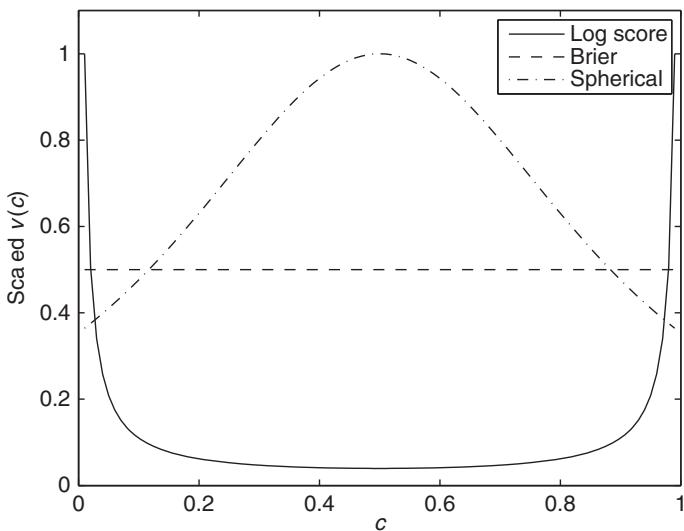
Figure 12.2: Weights for different scoring rules.

This relation was first shown in Shuford Jr, Albert, and Massengill (1966) and restated in Schervish (1989, Theorem 4.1). Schervish (1989) further showed that strictly proper scoring rules can be written as

$$U(y,p)=\{\begin{array}{ll}-{\int }_p^1(1-c)v(c)dc& \mathrm{for}y=1,\\ -{\int }_0^{p}cv(c)dc& \mathrm{for}y=0,\end{array}$$

where $v(c)>0$ for $c\in (0,1)$ . This equation interprets proper scoring rules as weighted averages of utility functions. Different choices of $v(c)$ yield different weighting functions. For example, setting $v(c)=[c(1-c){]}^{-1}$ results in the log score function— better known as the maximum likelihood objective function given a model for the conditional probability—whereas $v(c)=1$ yields the quadratic score. Notice the very different weights on these two scoring rules. The log score puts very high weights on individuals whose loss functions yield cutoffs close to 0 or 1 relative to those with loss functions that result in cutoffs near 0.5. The quadratic or Brier score (Brier, 1950) weighs all individuals evenly, while the spherical score weighs cutoffs close to 0.5 more heavily than cutoffs near the tail. The weights for the log score, Brier, and spherical scoring rules are shown in figure 12.2.

The relationship between the weights v(c) and the scoring rule can be shown to be

$$v(c)=\frac{\partial f_1(c)}{\partial c}\left(\frac{1}{1-c}\right).$$

These results hold for the conventional scoring rules applied to binary problems such as the log score, Brier score, and spherical score, all of which weigh utility functions symmetrically around $p=0.5$ . Moreover, the results can be employed to construct a variety of proper scoring rules that need not treat costs symmetrically.