正在学习
9.6 EMPIRICAL EXAMPLE
9.6 EMPIRICAL EXAMPLE
We next consider an empirical example based on a three-variable system comprising the CPI inflation rate, the unemployment rate, and the three-month T-bill rate. This small-scale VAR serves to illustrate some of the issues that arise in empirical forecasting with VAR models. Our analysis uses quarterly data over the period 1954Q1–2014Q4.
Figure 9.2 shows recursively generated forecasts of the US unemployment rate over the period 1970–2014. The graphs show forecasts from a BVAR with Minnesota priors, a VAR with lag length selected by AIC or BIC, a univariate autoregressive (AR) model with lag length selected by AIC, and forecasts from a fixed-lag
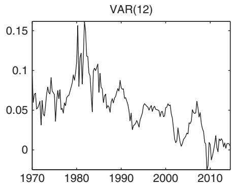
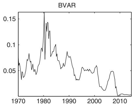
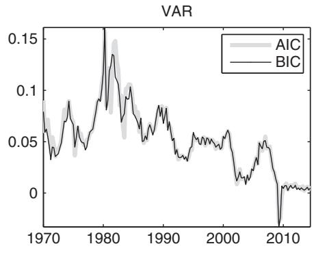
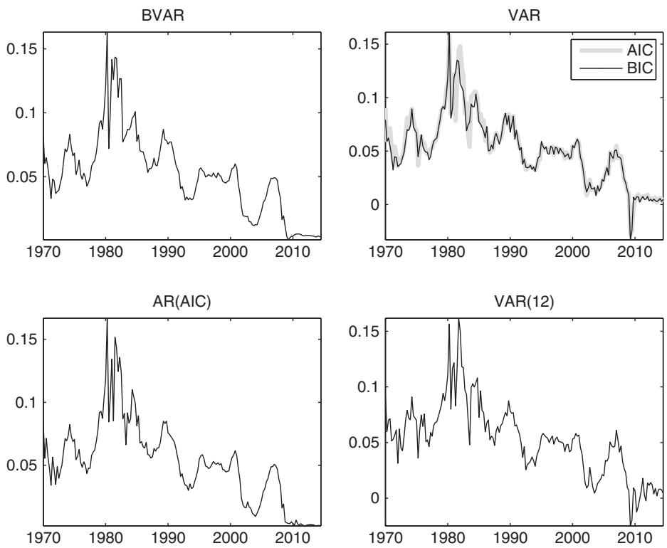
Figure 9.3: Recursive forecasts of the three-month T-bill rate. The figure shows forecasts of the three-month T-bill rate generated by a Bayesian VAR (BVAR), VARs with lag length selected by the AIC or BIC, a univariate AR with lag length selected by the AIC, and a VAR with 12 lags.
VAR(12). The forecasts are very similar with correlations ranging from 0.97 to 0.998, suggesting that for this variable how the lags are selected in the VAR makes little difference for the forecasts. Moreover, the similarity of the BVAR and AR forecasts suggests that past unemployment captures most of the predictability of future unemployment.
Similar conclusions emerge for the T-bill rate forecasts shown in figure 9.3. The forecasts from the BVAR, VAR, and AR models share a very similar trend although the individual forecasts differ on occasion, particularly towards the end of the sample where the extremely low interest rates result in near-zero forecasts for the BVAR and AR models, whereas the VAR models produce negative and more volatile forecasts during this period. Again the forecasts are very similar, with correlations ranging from 0.96 to 0.99.
Larger differences in forecasts are found for the inflation rate shown in figure 9.4. For example, notable differences emerge during 1980, which reflect the highly volatile interest rates, information on which is of course ignored by a purely autoregressive model for inflation. Only the VAR(12) model forecasts a sharp, but short-lived, decline in the inflation rate around 1983. Correlations across the various forecasts are now much smaller and range from 0.71 to 0.89.
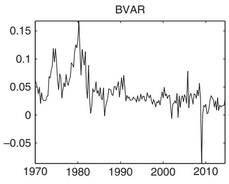
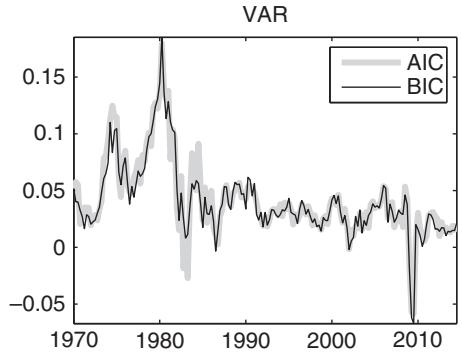
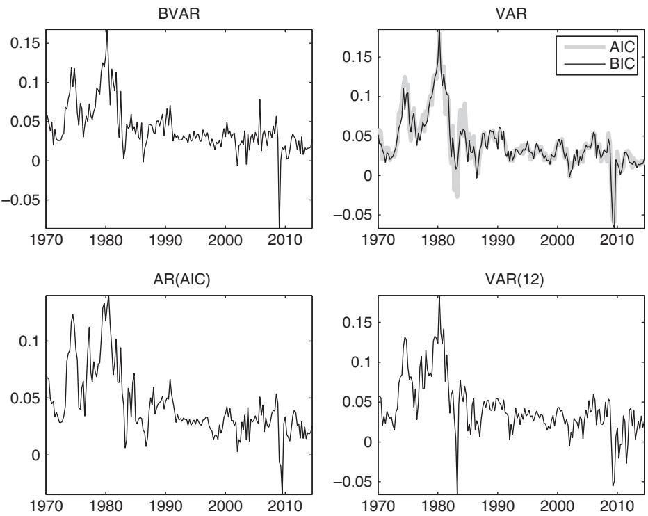
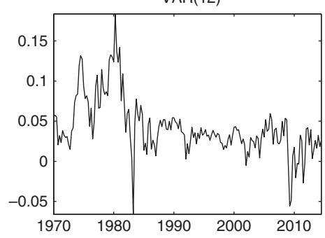
Figure 9.4: Recursive forecasts of the inflation rate. The figure shows forecasts of the inflation rate generated by a Bayesian VAR (BVAR), VARs with lag length selected by the AIC or BIC, a univariate autoregressive (AR) model with lag length selected by the AIC, and a VAR with 16 lags.
A key reason for the popularity of VARs is that they can be used to generate multistep forecasts. For a stationary VAR, the forecasts should converge to the steady-state value, the longer the forecast horizon, which will tend to smooth the forecasts. Figure 9.5 illustrates this effect at two separate points, namely for an initial value below the mean and an initial value above the mean. In both cases the forecast converges to the mean as the horizon is extended.
Figure 9.6 plots recursively generated one-, two-, four-, and eight-quarter-ahead forecasts of the unemployment rate generated by VAR(4) and VAR(12) models. Mean reversion in the long-horizon forecasts is clearly seen at the two longest horizons, although the persistence of the variables means that substantial time variation remains in the forecasts even at the eight-quarter horizon. The VAR(4) model generates smoother forecasts than the VAR(12) model, particularly at the four- and eight-quarter horizons.
Table 9.1 reports out-of-sample RMSE values for the various VAR models, using 1970–2014 as the evaluation period. For the unemployment rate, the best forecasts are generated by the BVAR model followed by the univariate autoregressive model with lag length selected by the AIC. The VAR(12) model generates particularly poor forecasts as does the random walk model (particularly at long horizons) which ignores mean reversion in the unemployment rate. Conversely, for the interest rates series the random walk forecasts are best, followed by the BVAR forecasts and the VAR forecasts with lag length selected by the BIC. Once again, methods that include the most lags and thus are most prone to estimation error such as the VAR(12) and the VAR with lag length selected by AIC, produce the least accurate forecasts. Finally, for the inflation series the univariate forecasts are best, followed by the BVAR forecasts. Again the least accurate forecasts are generated by the VAR(12) model.
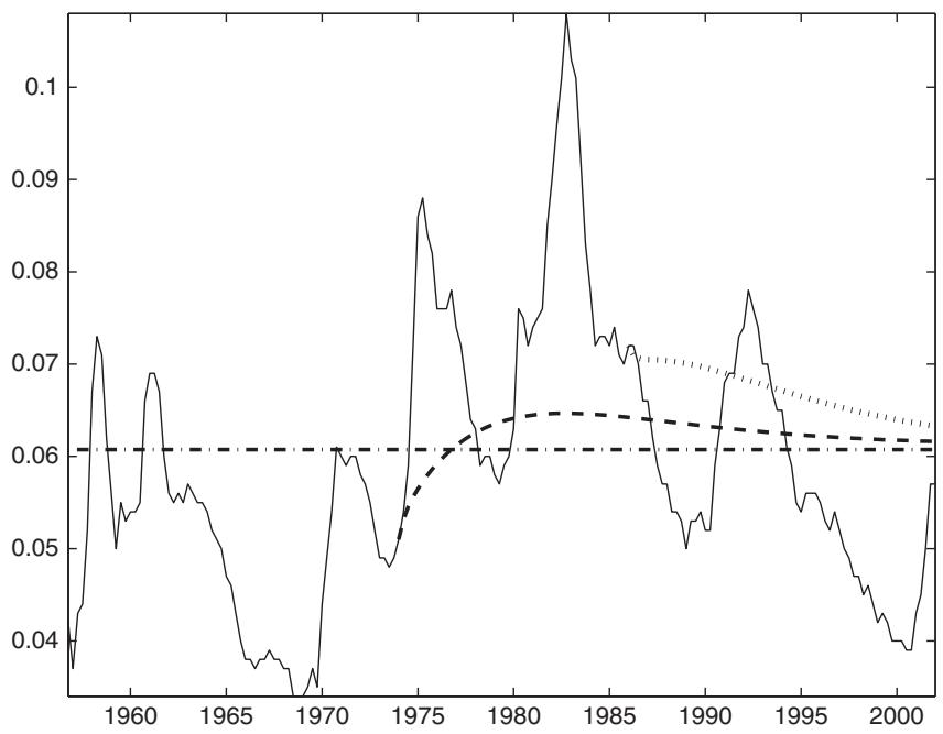
Figure 9.5: Mean reversion of multi-step-ahead forecasts of the unemployment rate generated at values above and below the average unemployment rate.
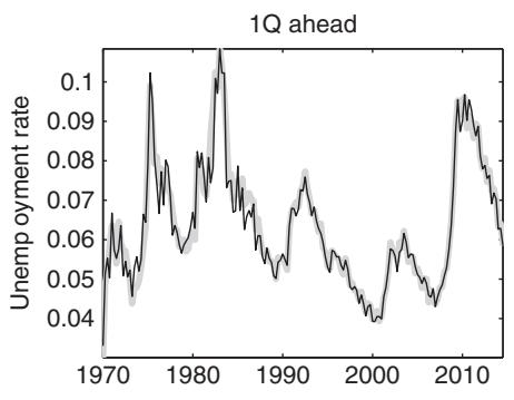
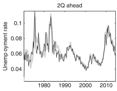
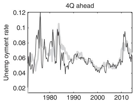
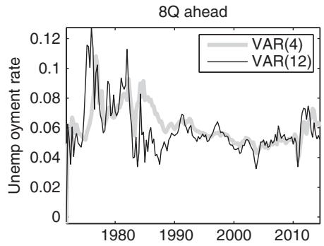
Figure 9.6: Recursive multi-step-ahead forecasts of the unemployment rate.
TABLE 9.1:
Root mean squared forecast errors from various VAR models fitted to a model comprising the quarterly unemployment rate, interest rate, and inflation rate.
| Steps | BVAR | VAR(AIC) | VAR(BIC) | VAR(4) | VAR(12) | AR(AIC) | RW |
| Unemployment rate | |||||||
| 1Q | 0.3322 | 0.4133 | 0.3543 | 0.3677 | 0.4772 | 0.3326 | 0.3799 |
| 2Q | 0.5750 | 0.7187 | 0.6097 | 0.6417 | 0.8295 | 0.5817 | 0.6635 |
| 4Q | 0.9941 | 1.2745 | 1.0644 | 1.1540 | 1.4694 | 1.0610 | 1.1423 |
| 8Q | 1.4114 | 1.7281 | 1.4693 | 1.6122 | 1.9049 | 1.5614 | 1.7617 |
| Interest rate | |||||||
| 1Q | 1.1489 | 1.3717 | 1.2117 | 1.2298 | 1.4554 | 1.2490 | 1.1038 |
| 2Q | 1.4845 | 1.6204 | 1.5309 | 1.5269 | 1.8346 | 1.5110 | 1.4045 |
| 4Q | 1.9263 | 2.2775 | 1.9702 | 2.0441 | 2.5018 | 2.0024 | 1.8264 |
| 8Q | 2.8213 | 3.5367 | 2.7966 | 3.1453 | 3.6461 | 2.9525 | 2.6779 |
| Inflation rate | |||||||
| 1Q | 2.7894 | 2.8939 | 2.7982 | 2.7417 | 2.9751 | 2.7221 | 3.1377 |
| 2Q | 2.9455 | 3.1772 | 3.1455 | 3.0765 | 3.3546 | 2.8400 | 3.3567 |
| 4Q | 3.1777 | 3.6610 | 3.3607 | 3.4140 | 3.8364 | 3.1344 | 3.5600 |
| 8Q | 4.1238 | 5.5776 | 4.5494 | 5.1039 | 4.9918 | 3.7780 | 4.1143 |
TABLE 9.2:
Diebold–Mariano test statistics for one-quarter-ahead squared error forecasting performance measured relative to the random walk benchmark.
| Method | Unemployment | Interest rate | Inflation rate |
| BVAR | 3.6023 | -1.3997 | -0.0579 |
| VAR(AIC) | -0.1369 | -3.0321 | -2.4497 |
| VAR(BIC) | 1.9550 | -0.7372 | -1.0005 |
| VAR(4) | 0.7274 | -2.2550 | -1.8303 |
| VAR(12) | -1.2952 | -3.2039 | -2.3156 |
| AR(AIC) | 1.7936 | -2.1504 | 0.8370 |
| Random walk | 0.0000 | 0.0000 | 0.0000 |
Table 9.2 reports values of the Diebold–Mariano test for equal MSE performance using the random walk forecasts as benchmark. The t-tests are set up so that positive values of the test statistic indicate that a particular forecasting method beats the random walk forecast, whereas negative values suggest that the benchmark is best. Only for the unemployment series do we find some evidence that the BVAR, VAR with AIC lag length selection, and the univariate autoregressive model outperforms the random walk.
These findings suggest that using an overparameterized model such as the VAR(12) specification can yield poor results. More parsimonious VAR models tend to do better—as witnessed by the tendency of VARs selected by the BIC to perform better than VARs selected by the AIC, and for some variables the parsimonious univariate autoregressive model performs well. Although the BVAR forecasts generally perform well, no single approach appears to be dominant across variables and forecast horizons, illustrating the need to adopt different approaches to different situations and perhaps also consider forecast combinations; see chapter 15.
练习题
Which of the following is NOT one of the variables in the empirical example's three-variable system?
What is the analysis data period for the empirical example?
Which of the following models were used to generate forecasts for the unemployment rate in the empirical example?
The VAR(12) model forecasts a sharp, but short-lived, decline in the inflation rate around 1983.
For a stationary VAR, the forecasts should converge to the steady-state value as the forecast horizon increases.
The forecasts for the unemployment rate from different models show correlations ranging from ___ to 0.998.
The forecasts for the inflation rate across various models have correlations ranging from 0.71 to ___.
Explain why the forecasts for the unemployment rate are very similar across different models.
What is the key reason for the popularity of VAR models in forecasting?
Which of the following statements are true regarding the forecast performance of different models for the interest rates series?
Which model generates smoother forecasts for the unemployment rate, particularly at the four- and eight-quarter horizons?
Which model generates particularly poor forecasts for the unemployment rate?
What is the main conclusion of Del Negro and Schorfheide (2013) regarding the predictive performance of DSGE models compared to VAR models?
Based on the empirical example in section 9.6, which of the following statements are true regarding the forecasts of different variables?
Explain why the VAR(12) model generates poor forecasts for the unemployment rate and inflation rate in the empirical example of section 9.6.
登录后解锁笔记、知识点解析、AI 问答
立即登录