正在学习
8.2.1 Empirical Evidence
8.2.1 Empirical Evidence
Empirical evidence generally does not suggest that these nonlinear univariate models systematically produce better forecasts than linear alternatives. In the forecasting experiment for US macroeconomic data conducted by Stock and Watson (1999), STAR models did not generally outperform linear models. Sarantis (1999) comes to the same conclusion in analyzing predictability of real exchange rates, while Kilian and Taylor (2003) find some evidence that exponential STAR models can predict exchange rates at 2–3 year horizons, though not at shorter horizons. Teräsvirta (2006) also concludes that there is relatively weak evidence that these models generate better point forecasts than competing methods, although he also concludes that these models have greater promise in density forecasting and can be useful as part of forecast combinations.
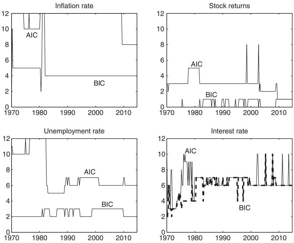
Figure 8.1: Recursive lag length selection for the smooth threshold autoregressive (STAR) model with two states.
Part of the reason for these findings is that these nonlinear models can be more sensitive to outliers in the data and so parameter estimation error is an important consideration, especially in small samples.
As an empirical illustration, using the quarterly data on inflation, stock returns, unemployment and interest rates from chapter 7, figure 8.1 plots the number of terms in the STAR model selected recursively from 1970 to 2010 using the AIC or BIC methods. For most of these series, once again, the AIC selects considerably more lags than the BIC. For example, for the inflation rate the AIC selects 12 lags most of the time, although this declines to 8 lags at the end of the sample. The BIC, meanwhile, selects 4 or 5 lags during most of the sample.
Figure 8.2 shows recursively generated forecasts generated by the STAR models with lag length selected by the AIC or BIC methods. The forecasts are mostly similar to those generated by the linear AR model although on some occasions these nonlinear models can generate quite extreme forecasts, as in the case of the inflation rate for which an extremely large negative forecast is generated in 1980 or for the T-bill rate where large negative forecasts are generated in the early eighties. The forecasts of stock returns generated by the models selected by the AIC are also notably more volatile than their linear counterparts in chapter 7 due in part to the inclusion of a larger number of terms by the STAR model.
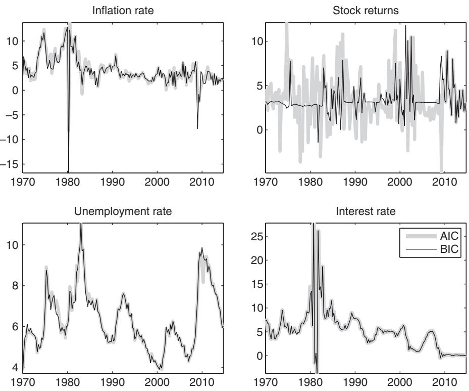
Figure 8.2: Recursive out-of-sample forecasts generated by smooth threshold autoregressive (STAR) models selected by the AIC or BIC.
8.3 REGIME SWITCHING MODELS
Since their introduction into economics by Hamilton (1989), Markov switching or regime switching models have become a popular class of models in economics and finance. Regime switching models share similarities with both TAR and STAR models. In common with these models, they introduce a number of regimes linked by a function that determines which regime occurs at a particular point in time. An example of a simple regime switching process with regime-dependent mean and variance is
where indicates the current regime. For example, with two regimes, y is normally distributed in regime 1 and normally distributed in regime 2. The difference between TAR or STAR models versus Markov switching models lies in how they determine the regime.
The Markov switching model assumes that the regime indicator is driven by an underlying Markov process. It is common to assume that the transition probabilities are constant through time and that transitions between regimes depend only on the previous regime and so are first-order Markov:
Since probabilities sum to 1 we need only define parameters for a subset of the probabilities. For the model with two regimes we can write the transition probability matrix as
Hence there are only two transition probabilities to model, equivalent to the probabilities of remaining within the same regime. The first-order homogenous Markov chain assumes that the transition probabilities do not depend on the data. For example if regime 1 is expansion and regime 2 is recession, the model has a constant probability of transiting from a recession to an expansion no matter how long the recession has been going on.
练习题
According to Stock and Watson (1999), which of the following statements is true about STAR models in forecasting US macroeconomic data?
What is one reason why nonlinear models may not generate better point forecasts than competing methods?
In the empirical illustration using quarterly data, which method selects more lags for the inflation rate?
Which of the following are true about the forecasts generated by STAR models with lag length selected by AIC or BIC?
Kilian and Taylor (2003) found that exponential STAR models can predict exchange rates at all horizons.
Teräsvirta (2006) concluded that nonlinear models have greater promise in density forecasting.
The AIC selects ___ lags for the inflation rate most of the time, although this declines to 8 lags at the end of the sample.
The BIC selects ___ lags during most of the sample for the inflation rate.
Explain why the forecasts of stock returns generated by STAR models selected by the AIC are more volatile than their linear counterparts.
What is the main difference between the forecasts generated by STAR models and linear AR models?
What is the key difference between Markov switching models and TAR/STAR models?
In a Markov switching model, what does the regime indicator represent?
Which of the following are true about the simple regime switching process described by the equation , where ?
The transition probabilities in a Markov switching model are assumed to be constant through time and depend only on the previous regime.
The first-order homogenous Markov chain assumes that transition probabilities depend on the data.
In a Markov switching model with two regimes, the transition probability matrix can be written as . There are only ___ transition probabilities to model.
Explain the difference between a first-order Markov process and a higher-order Markov process.
What is the significance of the first-order homogenous Markov chain assumption in regime switching models?
Which of the following statements are true about the sensitivity of nonlinear models to outliers and their impact on forecasting?
How do the forecasts generated by STAR models with lag length selected by AIC differ from those selected by BIC in terms of volatility and extremeness?
Which of the following statements is true regarding the empirical evidence on nonlinear univariate models versus linear models in forecasting US macroeconomic data?
Which of the following statements are true regarding the sensitivity of nonlinear models to outliers and the lag selection in STAR models using AIC and BIC?
The forecasts generated by STAR models with lag length selected by the AIC are generally less volatile than those generated by linear AR models.
The ___ model assumes that the regime indicator is driven by an underlying Markov process, and transitions between regimes depend only on the previous regime.
登录后解锁笔记、知识点解析、AI 问答
立即登录