7.1.2 ARMA Models

7.1.2 ARMA Models

As suggested by their name, autoregressive models specify Y as a function of its own lags, while moving average models specify Y as a function of an average of past shocks (innovations) to the series. Specifically, an $\mathrm{ARMA}(p,q)$ specification for a stationary variable ${\gamma }_t$ is a model whose highest-order autoregressive term is of pth order while the highest-order moving average term is of qth order so the model takes the following form:

$$y_t={\varphi }_1{y}_{t-1}+\cdot \cdot \cdot +{\varphi }_p{y}_{t-p}+{\epsilon }_t+{\theta }_1{\epsilon }_{t-1}+\cdot \cdot \cdot +{\theta }_q{\epsilon }_{t-q}.\text{\hspace{1em}(7.4)}$$

Equivalently, in power series notation,

$$\varphi (L)y_t=\theta (L){\epsilon }_t,\text{\hspace{1em}(7.5)}$$

where the lag polynomials take the form

$$\varphi (L)=1-\sum _{j=1}^P{\varphi }_i{L}^i,\text{\hspace{1em}(7.6)}$$

$$\theta (L)=\sum _{j=0}^q{\theta }_i{L}^i,\text{\hspace{1em}(7.7)}$$

and L is the lag operator, i.e., $L^j{y}_t=y_{t-j}$ for positive integers $j.$ . The innovation term ${\epsilon }_t$ in (7.4) or (7.5) is assumed to be a white noise process.

Example 7.1.3 (Forecast errors for the AR(1) model). Pure AR or MA models arise through simple restrictions on the ARMA parameters in (7.4). The simplest and most common ARMA process is the ARMA(1,0) or $AR(1)$ model which has no moving average terms:

$$y_t={\varphi }_1{y}_{t-1}+{\epsilon }_t,\text{\hspace{1em}(7.8)}$$

$or,$ in lag polynomial notation, $(1-{\varphi }_{1}L)y_t={\epsilon }_t,\theta (L)=1$

By backward substitution,

$$y_t={\varphi }_1(\underset{y_{t-1}}{\underbrace{{\varphi }_1{y}_{t-2}+{\epsilon }_{t-1}}})+{\epsilon }_t={\varphi }_1^2{y}_{t-2}+{\epsilon }_t+{\varphi }_1{\epsilon }_{t-1}.$$

Iterating further backwards, we have, for $h\ge 1$

$$\begin{array}{l}{y}_t={\varphi }_1^h{y}_{t-h}+\sum _{s=0}^{h-1}{\varphi }_1^s{\epsilon }_{t-s}\\ ={\varphi }_1^h{y}_{t-h}+\theta (L){\epsilon }_t,\end{array}\text{\hspace{1em}(7.9)}$$

where the elements of the lag polynomial $\theta (L)$ are ${\theta }_i={\varphi }_1^i$ . Further iterations result in the order of the polynomial $\theta (L)$ becoming larger and larger and so the $AR(1)$ model is equivalent to an $MA(\infty )$ model as long as ${\varphi }_1^k{y}_{t-k}$ becomes “small” in a mean squared sense. To see what this implies for the $AR(1)$ model, note that

$$E[y_t-\sum _{s=0}^{h-1}{\varphi }_1^s{\epsilon }_{t-s}{]}^2=E[{\varphi }_1^h{y}_{t-h}{]}^2\le {\varphi }_1^{2h}{\gamma }_y(0)0\text{\hspace{1em}(7.10)}$$

as $h\infty$ , provided that ${\varphi }_1^{2h}0$ . This condition is satisfied $if|{\varphi }_1|<1$ holds. Hence, the $AR(1)$ process has an equivalent $MA(\infty )$ representation provided that ${\varphi }_1^{2h}0;$ which is thus the stationarity condition for this process.

Example 7.1.4 (AR representation of the MA(1) process). A second example is the ARMA(0,1) or MA(1) model

$$y_t={\epsilon }_t+{\theta }_1{\epsilon }_{t-1},\text{\hspace{1em}(7.11)}$$

where now $\varphi (L)=1,\theta (L)=1+{\theta }_{1}L$ . Again we can construct an infinite-order AR process from this MA(1) process. Backwards substitution in (7.11) yields

$${\epsilon }_t=\sum _{s=0}^h(-{\theta }_1{)}^s{y}_{t-s}+(-{\theta }_1{)}^{h+1}{\epsilon }_{t-h-1}.\text{\hspace{1em}(7.12)}$$

Once again, in a mean squared sense ${\gamma }_t$ becomes equivalent to an AR(h) process with coefficients ${\varphi }_s=(-{\theta }_1{)}^s$ provided that $\bar{E}\left[(-{\theta }_1{)}^h\overline{{\epsilon }_{t-h}}\right]$ gets small as h increases. Letting $h\infty ,\mathcal{E}[(-{\theta }_1{)}^h{\epsilon }_{t-h}{]}^2=(-{\theta }_1{)}^h{\sigma }^{2}0$ provided that $|{\theta }_1|<1$ . This condition, $|{\theta }_1|<1$ , is known as invertibility. Hence, an invertible MA(1) process is equivalent to an infinite-order AR process.

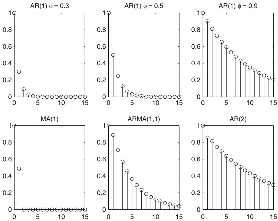
Figure 7.1: Population values of autocorrelations for different ARMA processes.

The stationarity condition for the AR(1) process $|{\varphi }_1|<1$ can be thought of in terms of the roots of the power series for the polynomial $\varphi (z)=1-{\varphi }_{1}z.$ . The root of this polynomial is ${\varphi }_1^{-1}$ and so $|{\varphi }_1|<1$ means that the root is greater than 1. This is a necessary and sufficient condition for stationarity of an AR(1) process. More generally, stationarity of an $\mathrm{AR}(p)$ model requires that all roots of the polynomial $\varphi (z)$ fall outside the unit circle. The invertibility condition for $\theta (z)$ is similar. For the MA(1) case $|{\theta }_1|<1$ is equivalent to the condition that the root of the polynomial $\theta (z)=1+{\theta }_{1}z$ is greater than 1. More generally for an $\mathrm{MA}(q)$ model the roots of $\theta (z)$ must be outside the unit circle for invertibility to be satisfied. Thus, an $\mathrm{ARMA}(p,q)$ process that is stationary and invertible can be written either as an AR model or as an MA model, typically of infinite order. In power series notation, we have either $y_t=\varphi (L{)}^{-1}\theta (L){\epsilon }_t\mathrm{or}\theta (L{)}^{-1}\varphi (L)y_t={\epsilon }_t$

To obtain intuition for the ARMA models, it is useful to consider the autocorrelations for some specific models. Figure 7.1 plots the population autocorrelations, $\gamma (j)$ , for AR(1) processes with ${\varphi }_1=0.3,0.5,0.9$ , an MA(1) process with ${\theta }_1=0.8$ , an $\mathrm{ARMA}(1,1)$ process with $({\varphi }_1,{\theta }_1)=(0.8,0.5)$ , and an AR(2) process with $({\varphi }_1,{\varphi }_2)=$ (0.6, 0.3). In all cases the autocorrelations taper off as the horizon gets extended. This is a consequence of stationarity. For stationary processes, as $h\infty ,$ the forecast $f_{T+h|T}\to E\left[y_{T+h}\right]$ converges to the unconditional mean (assumed to be 0 here) and so the MSE converges to the unconditional variance, $\mathrm{Var}(y_T)$ . This mean-reverting property is important to bear in mind when considering the limitations of ARMA forecasts. These models will never generate expected values that are further away from the long-run (steady-state) mean than the current value.

There are large differences in the autocorrelation patterns shown in figure 7.1. Since the autocorrelations of the AR(1) processes are ${\varphi }_1^h$ , these processes display stronger autocorrelations, the larger is ${\varphi }_1$ . The autocorrelation of the AR(2) process is quite similar to the AR(1) process with ${\varphi }_1=0.9$ . Conversely, the MA(1) process has very short memory. Compared with the AR(1) process, the autocorrelations of the ARMA(1,1) process get an extra “bump” in the first-order autocorrelation, but decay exponentially for higher-order autocorrelations.

One way to identify a forecasting model for a given time series is by comparing its autocorrelations with plots of known processes such as those shown in figure 7.1. To illustrate how this works, consider four variables, namely the rate of inflation, stock returns, the unemployment rate, and the three-month T-bill rate, all measured at a quarterly horizon. The inflation rate is defined as $\Delta \log ({\mathrm{CPIAUCSL}}_{t+1}/{\mathrm{CPIAUCSL}}_t)$ , where CPIAUCSL is the Consumer Price Index for All Urban Consumers: All Items, available from the FRED database maintained by the Federal Reserve Bank of St. Louis. Stock returns are measured as the valueweighted return (including dividends) on stocks traded on the NYSE, AMEX, and NASDAQ exchanges and are obtained from Welch and Goyal (2008). The unemployment rate is taken from FRED. The interest rate is the three-month Treasury Bill rate (secondary market, TB3MS) and is also available from the FRED database. Our data sample runs from 1947Q1 through 2014Q4.

Figure 7.2 provides time-series plots of these four variables, while figure 7.3 shows the sample estimates of their autocorrelations along with standard error bands. The interest rate series in particular, but also the unemployment rate, is highly persistent with autocorrelations that decay very slowly. The inflation rate is modestly persistent with a first-order autocorrelation estimate around 0.6, followed by a gradual decay in higher-order autocorrelations. Unemployment rates and, especially, interest rates have low-order autocorrelations that exceed 0.9 and the autocorrelations of the interest rate series exceed 0.2 even after 40 quarters. Stock returns, on the other hand, are not serially correlated at all with autocorrelations fluctuating around 0 and no systematic patterns in signs or magnitudes.

The Wold representation theorem states that MA(∞) processes can be used to represent the first two moments of any covariance stationary process. In practice, we cannot estimate an infinite set of MA coefficients and so instead use finite order ARMA models. These can be viewed as approximations to such MA(∞) processes. ARMA models are based on linear projections which provide reasonable forecasts of linear processes under MSE loss. AR models are particularly popular in forecasting in part because, for any forecast horizon, $h>0;$ , they can be estimated by least squares by projecting $Y_{t+h}$ on $\{Y_{t-j}{\}}_{j=0}^{\infty }{}_{:}$ , regardless of stationarity of the data-generating process. This does not ensure, however, that the coefficients on the AR model remain constant over time, nor does it suggest that a finite-order AR or ARMA approximation is appropriate. This matters since we never observe the infinite past.

Second, the Wold representation theorem establishes that we can write any covariance stationary process as an MA process, possibly of infinite order. ARMA models fill out or exhaust the set of all possible linear models that capture the first two moments (mean and covariances) of a covariance stationary process. Further, from the Wold representation theorem, we are guaranteed that the coefficients on the lagged values of ${\gamma }_t$ and ${\epsilon }_t$ are constant. This result, along with their appealing simplicity, suggest that ARMA models will be practically useful for forecasting many economic time series.

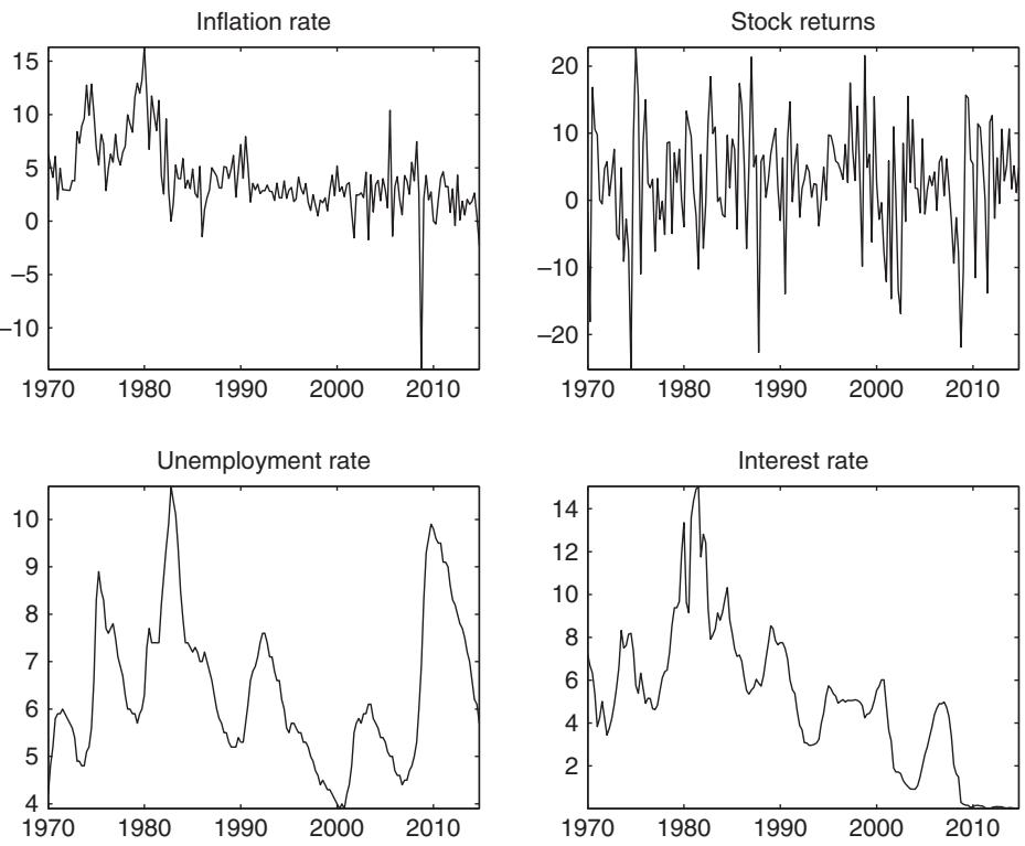
Figure 7.2: Time-series plots of the quarterly inflation rate, stock returns, unemployment rate, and interest rate.

None of this excludes the possibility that there is a nonlinear model of past data that provides a better predictor. Under MSE loss the best predictor is the conditional mean, which need not be a linear function of the past. We cover nonlinear models in more detail in chapter 8 but illustrate the point here through a simple example.

Example 7.1.5 (Bilinear process). Consider the bilinear process studied by Granger and Andersen (1978):

$$y_{t+1}=\beta {\epsilon }_t{y}_{t-1}+{\epsilon }_{t+1},{\epsilon }_{t+1}\sim iid(0,{\sigma }^2).$$

The autocorrelations of this process are 0 at all lags:

$$\begin{array}{rl}& \\ & E\left[y_{t+1}{y}_t\right]=E\left[(\beta {\epsilon }_t{y}_{t-1}+{\epsilon }_{t+1})(\beta {\epsilon }_{t-1}{y}_{t-2}+{\epsilon }_t)\right]\\ & \\ & =\beta E\left[{\epsilon }_t^2{y}_{t-1}\right]=\beta {\sigma }^{2}E\left[y_{t-1}\right]=0,\end{array}$$

$$E\left[y_{t+1}{y}_{t-1}\right]=E\left[(\beta {\epsilon }_t{y}_{t-1}+{\epsilon }_{t+1})(\beta {\epsilon }_{t-2}{y}_{t-3}+{\epsilon }_{t-1})\right]=0.$$

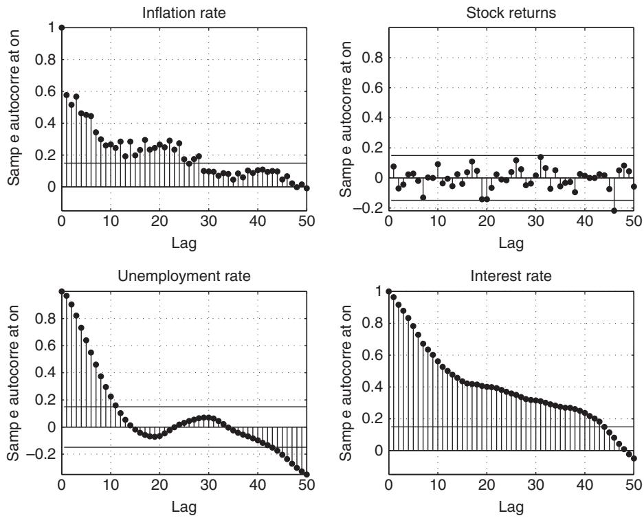
Figure 7.3: Quarterly sample autocorrelations for four economic variables.

Here we used that $E\left[{\epsilon }_t{\epsilon }_{t-j}\right]=0$ for all $j\ne 0$ . This means that the series cannot be predicted by means of linear forecasting models. Assuming that current and past values of y and ε are in the forecaster’s information set, so $Z_t=\{y_t,{\epsilon }_t,y_{t-1},{\epsilon }_{t-1},...\}$ however, a nonlinear model will be able to forecast $y_{t+1}$ since

$$E\left[y_{t+1}|Z_t\right]=\beta {\epsilon }_t{y}_{t-1},\text{\hspace{1em}(7.13)}$$

which is generally nonzero.