6.9 RISK FOR MODEL SELECTION METHODS: MONTE CARLO SIMULATIONS

6.9 RISK FOR MODEL SELECTION METHODS: MONTE CARLO SIMULATIONS

Model selection methods should be considered part of the estimation process. This leads us to focus on the risk of the forecast method as a function of the selection rule, the set of models under consideration, the data, and the true model parameters. For example, with two models and a statistic $\phi (z)=\{0,1\}$ , where 0 indicates choosing the first model and 1 indicates choosing the second model, the forecast generated by a model selection method can be written as

$$f^{\mathrm{MS}}(z)=f_1(z_t,{\hat{\beta }}_1)(1-\phi (z))+f_2(z_t,{\hat{\beta }}_2)\phi (z).\text{\hspace{1em}(6.43)}$$

The forecast associated with a model selection procedure is simply a more complicated function of the data than either of the individual models. However, it remains a function of the data and hence has a risk function that depends on the parameters of the true model, θ. A good model selection procedure delivers tolerable risk over reasonable models that are not obviously misspecified. The consistency criterion examines risk in the sense that it focuses on minimizing pointwise asymptotic risk when the true model lies in the set of candidate models. Asymptotic efficiency focuses on the limit of relative risk when the true model is larger than any of the candidate models. Each of these properties is asymptotic. Small sample evaluations of risk show that consistent model selection methods will not generally choose the correct model with probability 1. Methods that asymptotically are as good as the best model will not always be as good as the best model in small samples. Because of this, it is constructive to examine the risk functions of some popular methods in a Monte Carlo setting.

Another reason for considering Monte Carlo experiments is that risk functions associated with forecasts based on the model selection methods covered in this chapter are generally very difficult to characterize analytically. The reason is that the selected forecasts are not smooth functions of the underlying data, as is clear from (6.43), and risk depends heavily on the parameters of the forecasting model.

The first Monte Carlo simulation examines estimation of the mean for i.i.d. data generated as

$$y_t=\mu +{\epsilon }_t,{\epsilon }_t\sim \mathrm{ind}\mathrm{N}(0,1).\text{\hspace{1em}(6.44)}$$

Under MSE loss the best possible—but infeasible—estimator is to know the mean, $\mu$ , which results in a risk of 1, i.e., the variance of the unpredictable component, ${\epsilon }_t$ . Estimation of the mean, based on the sample average, results in a risk equal to $(1+T^{-1})$ , where $T$ is the sample size. In addition to simply using the sample mean, we can employ the model selection methods discussed above to choose between the model that either fixes the mean at $\mu =0$ (and hence involves no estimation error) or instead uses the sample mean, ${\bar{y}}_t$ , as the forecast. The methods we employ are (i) AIC; (ii) BIC; (iii) a pre-test method based on a t-test with a two-sided alternative and a size of 5%; (iv) Bagging of the loss minimization method in (iii), using an i.i.d. bootstrap that samples with replacement from the demeaned data.

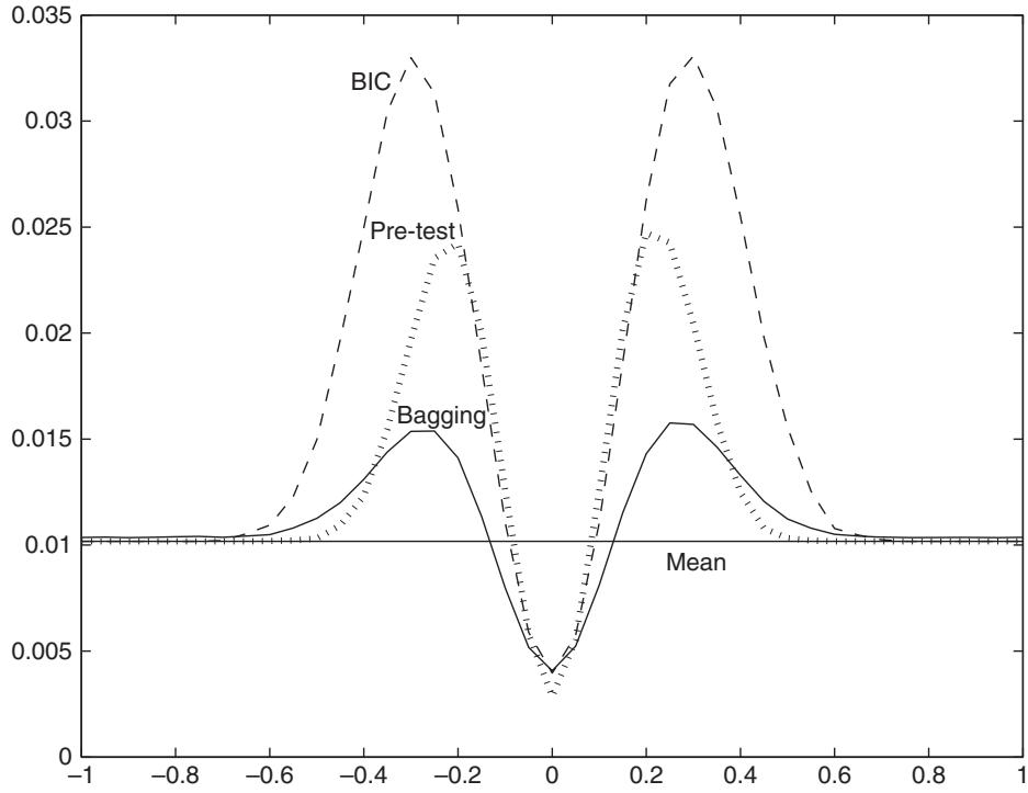
Figure 6.7: Estimation-related risk under different model selection methods for the model with a constant mean, $\mu ,$ and no time-varying predictors. The horizontal axis shows the magnitude of the mean, $\mu ,$ , while the vertical axis shows the estimationrelated risk.

Figure 6.7 shows the approximate estimation-related risk for four of these methods using a sample size of $T=100$ . The estimation-related risk removes firstorder uncertainty by removing the unpredictable component. Here this amounts to subtracting 1 from the risk. When the true mean is near ${}^{0,}$ in this example each of the model selection methods has a lower risk than that of simply estimating the mean. This happens because the model selection methods have a nonzero probability of choosing the forecast that imposes a zero mean. They do not always choose the correct model with $\mu =0$ , however, which is why none of the methods attain a zero estimation-related risk. The different values of risk at $\mu =0$ reflect the probability that the model with no mean is chosen.

Such gains from applying model selection methods when the true model has $\mu =0$ come at a cost, though, since all model selection methods have risk well above that of simply using the sample mean to forecast $\mathbf{y}$ when $\mu$ is “small,” i.e., close but not exactly equal to 0. In this neighborhood the risk rises above that of simply using the sample mean because the probability of choosing the (incorrect) model that imposes $\mu =0$ is nontrivial, which adversely impacts the MSE. This region of the parameter space is exactly where the tests have difficulties distinguishing between the two models. Eventually, though, as the true mean gets larger, each of the model selection methods chooses the model with a nonzero mean with probability 1 and the risk again declines to that of simply estimating the sample mean.

This “hump” in the risk function is ignored by the pointwise proofs discussed earlier—asymptotically at any point where $\mu \ne 0$ , the risk function converges to 0 pointwise. The hump never disappears, however, and there will always be a region near $\mu =0$ , where the model selection methods do not choose either model with probability 1, and hence there is always the chance that the risk induced by model selection will be higher than when the larger model is used. Hence, the uniform convergence results are not just of theoretical interest but also have practical value.

When more models are included in the search and coefficients are local to $0{,}^{15}$ analogous results can be obtained. Consider forecasting an outcome variable with $n_K=8$ possible regressors. The regressors are assumed to be independent of each other and are linked to the dependent variable through a linear model with coefficient vector ${\beta }_0$ . Let $n_{k_0}$ coefficients be equal to $\mu /\sqrt{n_{k_0}T}$ , where $T$ is the length of the estimation sample, which we again set to 100. The remaining coefficients are set to 0, so the data-generating process is

$$y_{t+1}=\sum _{i=1}^{n_{k_0}}\frac{\mu }{\sqrt{n_{k_0}T}}{x}_{it}+{\epsilon }_{t+1},{\epsilon }_{t+1}\sim \mathrm{ind}\mathrm{N}(0,1).$$

The full model uses all eight regressors. When $\mu \ne 0;$ the correctly specified regression includes only those variables that correspond to the $n_{k_0}$ nonzero coefficients. We consider sequential hypothesis tests, removing all variables with t-statistics that fail to reject a two-sided significance test at the 5% level, along with the BIC and AIC. Figure 6.8 reports results when $n_{k_0}=3.$ , so the majority of variables should be excluded, while figure 6.9 repeats the same exercise with $n_{k_0}=7$ , so only one variable needs to be excluded.

Figure 6.8 shows that the “hump” near 0 carries over to more complicated situations. Indeed, the only question is how big the hump is. Model selection methods can now perform worse than the kitchen sink approach that includes all—useful and useless—regressors. Even so, for most of the parameter space, the model selection methods outperform the kitchen sink approach which explains why model selection techniques are popular in practice. Moreover, the model selection procedures do even better than the correct specification when $\mu$ is sufficiently close to 0. This happens because model selection procedures are essentially shrinkage estimators, so when $\mu$ is close to 0, shrinkage becomes a useful approach.

In this example the AIC has very different properties to the BIC and the sequential testing approach. AIC does not perform so well when the other approaches do well, and does not do as poorly when the other approaches are poor. This is a consequence of the overfitting described above. When too many variables are included, the coefficient estimates do not get shrunk as much, and we are closer to the solution that includes all regressors and has a flat risk function. As μ gets larger, none of the methods are as good as including only the correct regressors. Despite the BIC’s property of correct asymptotic model selection, in small samples this method still appears to overfit somewhat. The overfitting is not as severe as that of the AIC, which also overfits asymptotically. In this experiment the sequential hypothesis test procedure is close to the BIC, but in larger samples the loss function of the BIC will get closer to that of the correct specification.

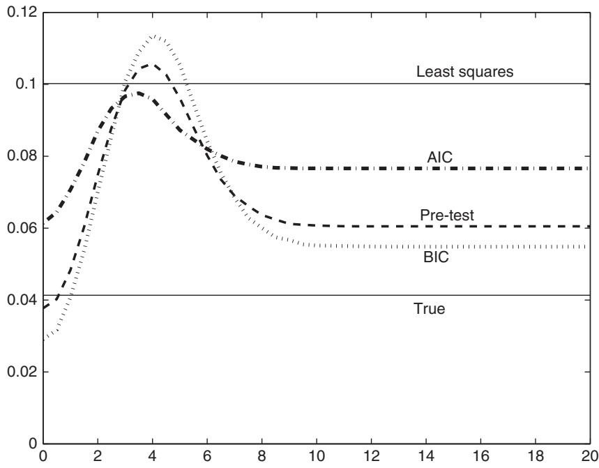
Figure 6.8: Estimation-related risk under different model selection methods for the model with eight time-varying predictors, three of which have nonzero coefficients. The horizontal axis shows the magnitude of the nonzero coefficients for the three predictor variables, while the vertical axis shows the estimation-related risk.

When nearly all the variables are to be included, the difference between the true model and the model that includes all variables is obviously small, as shown in figure 6.9. The effect of not needing to exclude many variables is threefold. First, the gains from model selection get larger when the coefficients are very close to 0. Second, the size of the hump in expected loss is larger for coefficients further away from 0. Third, when the coefficients are sufficiently far from 0, all of the methods perform similarly since the range of possibilities is small. The ordering of the size of the hump and the eventual point at which the methods settle down as μ gets larger is the same across all methods, however.

Despite these results, pre-test methods do have some valuable properties compared to simply using the underlying models. For large enough values of the nonzero parameters, asymptotically the pre-test estimator has the same risk as the largest model included in the set of models over which the search is conducted. This follows directly from the property that pre-tests are consistent, and hence the model preferred by the sequential search will be the largest model and so they have the same risk function. This prevents the risk function from increasing beyond bounds due to wrong exclusion of variables whose parameters are far away from 0. Contrast this with shrinkage methods which do not have such a property. This might not be as comforting as it seems, however, as it guarantees only that pre-testing performs well when it is obvious that some parameters are nonzero—a situation where shrinkage towards 0 is unlikely to be a sensible approach anyway.

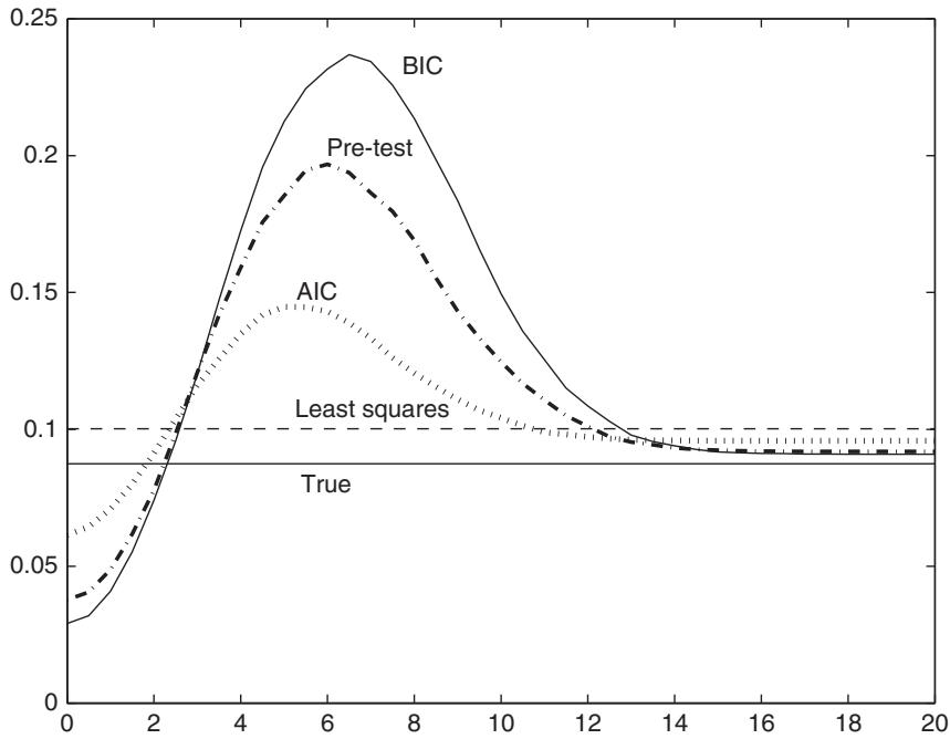
Figure 6.9: Estimation-related risk under different model selection methods for the model with eight time-varying predictors, seven of which have nonzero coefficients. The horizontal axis shows the magnitude of the nonzero coefficients for the seven predictor variables, while the vertical axis shows the estimation-related risk.

The results here are consistent with the findings in Ng (2013) that neither of the BIC or AIC criteria systematically dominate the other when it comes to evaluating the finite-sample risk of the associated forecasts. Using Monte Carlo simulations, Ng (2013) find that small models (models with few parameters to estimate) are not necessarily better than large models even if the data are generated by a model with a finite number of parameters. There is no way of getting around the problem that the best procedure will depend on the true data-generating process which in practice remains unknown.