正在学习
6.7.2 Economic Measures of Forecast Performance
6.7.2 Economic Measures of Forecast Performance
We have emphasized the potential for differences between statistical and economic measures of predictive performance. To evaluate this issue in the present context, we consider the portfolio allocation decisions of an investor with mean–variance preferences
where is the expected portfolio return, is the conditional variance of the portfolio return and captures the investor’s risk aversion. The investor chooses between a risk-free asset paying the three-month T-bill rate and the risky stock market portfolio. This investor’s portfolio return is given by , where is the risk-free rate, is the excess returns on stocks, net of the T-bill rate, and ωt is the weight on stocks selected on the basis of information available at time t, . To avoid bankruptcy concerns, we restrict to lie between 0 and 1 and so rule out short selling and leverage. The portfolio weight is then determined from , where is the recursively estimated OLS estimate from a linear return regression model and is the recursive estimate of the variance of the residuals from this regression.
Table 6.3 shows the mean return and volatility (standard deviation) of the resulting portfolio, along with the annualized certainty equivalent return (CER) and Sharpe ratio. The CER is defined as the annualized risk-free return which, over the evaluation sample, would have made an investor indifferent between following the benchmark strategy suggested by the prevailing mean model that assumes constant mean returns versus alternative strategies based on time-varying predictors.
TABLE 6.3:
Portfolio performance based on out-of-sample forecasts of quarterly US stock market returns using the forecasting methods listed in the rows. The portfolio performance is reported for a risk-averse mean–variance investor who chooses between stocks and T-bills based on the predicted excess return on stocks. Mean return and Std measure the mean and volatility of the resulting portfolio returns while CER is the certainty equivalent return and Sharpe is the Sharpe ratio. All measures are annualized.
| Method | Mean ret(%) | Std ret(%) | CER(%) | Sharpe(%) |
| AIC | 9.2573 | 23.5458 | 0.5687 | 0.3910 |
| BIC | 9.5058 | 22.4110 | 1.1431 | 0.4218 |
| Forward step | 8.9747 | 24.2177 | 0.0855 | 0.3684 |
| Backward step | 9.2020 | 20.7854 | 1.2782 | 0.4402 |
| Bagging α = 1% | 9.2130 | 24.1032 | 0.3584 | 0.3801 |
| Bagging | 9.6601 | 23.7252 | 0.9185 | 0.4050 |
| Lasso | 9.7686 | 23.2203 | 1.1751 | 0.4185 |
| Lasso | 9.6491 | 20.9934 | 1.6710 | 0.4572 |
| Cross valid | 8.3885 | 19.0016 | 0.9083 | 0.4387 |
| Prevailing mean | 8.9905 | 24.5500 | 0.0000 | 0.3641 |
The Sharpe ratio is the mean portfolio return in excess of the T-bill rate divided by the standard deviation of the portfolio return, both estimated over the evaluation sample.
The results suggest that the methods associated with the most volatile return forecasts do not always translate into portfolio strategies with more volatile returns. In fact, the most volatile portfolio returns are associated with the excess return forecasts that are mostly positive, i.e., the Bagging and Lasso methods with the smallest penalty factor, the AIC, and the prevailing mean. These methods do not, however, generate the highest certainty equivalent returns. The BIC, backward stepwise method, and the two Lasso methods generate CER values above 1% and Sharpe ratios somewhat higher than the Sharpe ratio associated with the prevailing mean model.
Figure 6.4 plots the recursively estimated allocation to stocks. This is the forecaster’s choice variable in this setting. A value of 1 corresponds to allocating all money to stocks, while a value of 0 corresponds to holding only T-bills. The portfolio weights fluctuate a great deal and frequently fall on the 0–1 bounds that we impose in our analysis. This is a result of our assumption of no transaction costs and would change if we assumed that large changes to the portfolio weights were costly. The upper bound of 100% invested in stocks is binding more often than the lower bound of zero allocation to stocks. This is a reflection of the equity risk premium, i.e., the higher historical mean of stock returns compared with returns on T-bills, whose average is positive during the sample and so it takes relatively strong evidence to persuade the investor not to allocate any money to stocks.
Figure 6.5 (left) shows a scatterplot of the RMSE versus the hit rate, i.e., the proportion of correctly predicted signs of excess returns, across the nine different model selection methods considered here. There is a negative correlation between the two measures, suggesting that the models with the highest proportion of correctly predicted signs tend to generate the smallest RMSE values.
Figure 6.5 (right) shows the potential disconnect between statistical measures of forecast performance such as RMSE and economic measures such as the CER.
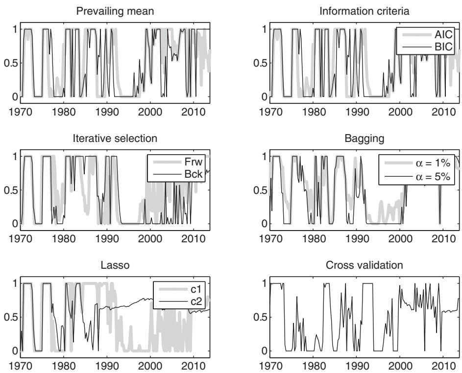
Figure 6.4: Mean–variance investor’s allocation to stocks based on recursively generated predictions using different ways to select the forecasting model. A value of 1 on the vertical axis shows a 100% allocation to stocks, while 0 shows a 100% allocation to Treasury bills.
Interestingly, the methods with the highest RMSE values tend to generate the highest CER values. For example, the models selected by the BIC and backward stepwise methods both generate high RMSE values, but also generate mean CER estimates of 1% per year or higher.
These findings suggest that forecasting methods with poor statistical performance can still yield forecasts that are valuable from an economic perspective. The reason is that large forecast errors can be punished more heavily by convex statistical loss functions such as MSE compared with economic loss functions which may put less weight on the large forecast errors.
Figure 6.6 plots the cumulative wealth over time from investing 1 in 1970 and then using the recursively generated forecasts to optimally allocate between the stock market portfolio and three-month T-bills. We show results for the prevailing mean strategy which does not model any time variation in the conditional equity risk premium. This strategy ends up with \35 in 2013. The best performing strategy is the Lasso method using the larger penalty term (c2) which generates a cumulated wealth above $50 at the end of 2013. Such plots should be interpreted with caution given the wide standard errors that surround the cumulative values. Nevertheless, they do serve as an illustration that economic and statistical measures of forecasting performance can yield quite different results.
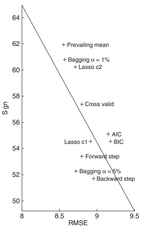
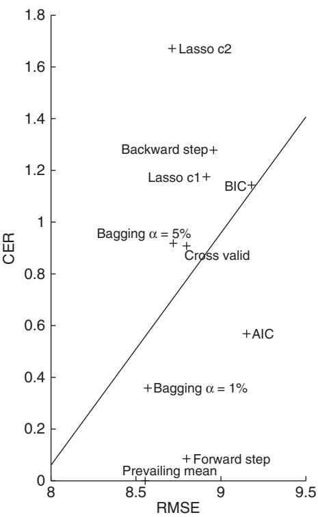
Figure 6.5: Relation between the percentage of correctly predicted signs of excess stock returns versus the root mean squared error (RMSE) (left) and the relation between a mean–variance investor’s certainty equivalent return (CER) versus the RMSE (right).
练习题
What does the investor's mean-variance preferences formula represent?
Which method in Table 6.3 has the highest Sharpe ratio?
Which methods generate CER values above 1% according to Table 6.3?
Which methods are associated with the most volatile portfolio returns according to the source material?
The portfolio weight determination formula ensures that the portfolio weight lies between 0 and 1.
The prevailing mean model generates the highest CER value according to Table 6.3.
The Sharpe ratio is defined as the mean portfolio return in excess of the T-bill rate divided by the ___.
The CER is defined as the annualized risk-free return which would have made an investor indifferent between following the benchmark strategy suggested by the prevailing mean model and alternative strategies based on ___.
Explain why the portfolio weights fluctuate a great deal and frequently fall on the 0–1 bounds.
How does the Lasso method's penalty factor influence the volatility of the forecasts?
Which of the following statements is true about the portfolio weight determination formula ?
Which of the following methods are associated with higher certainty equivalent returns (CER) according to Table 6.3?
The CER is defined as the annualized risk-free return which, over the evaluation sample, would have made an investor indifferent between following the benchmark strategy suggested by the ___ model and alternative strategies based on time-varying predictors.
Explain how the portfolio weight is determined and why it is restricted to lie between 0 and 1.
登录后解锁笔记、知识点解析、AI 问答
立即登录