正在学习
6.7.1 Statistical Measures of Forecast Performance
6.7.1 Statistical Measures of Forecast Performance
We study out-of-sample results even though the methods we use are based on penalized in-sample performance. In part, this is because we wish to see how much the selected forecasting models change over time and across different economic environments. A second reason is that this allows us to simulate the forecasting models’ “real-time” performance. The advantages and disadvantages of this approach are discussed in more detail in chapter 17 of the book.
All methods considered here use linear forecasting models. The forward stepwise approach uses a maximum p-value of 0.05 for a predictor to be added to the existing forecasting model. The backward stepwise approach uses a minimum p-value of 0.10 for a predictor to be removed from the existing model.
For the Lasso method, we choose two very small values of the penalty factor, λ. Specifically, we use the formula of Belloni and Chernozhukov (2011),√ , setting (which we label and (labeled
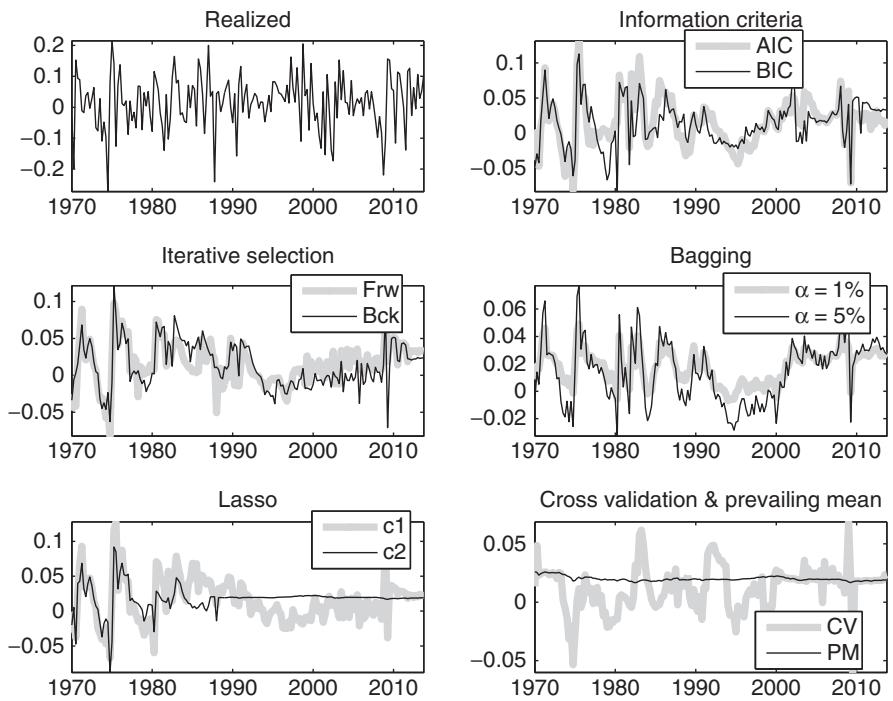
Figure 6.2: Quarterly US stock market returns and recursively generated out-of-sample forecasts based on a variety of forecasting and model selection methods, including the AIC and BIC information criteria, forward (frw) and backward (bck) stepwise selection, Bagging with different significance levels, Lasso with different penalties, cross validation (CV), and the prevailing mean (PM).
Our implementation of the Bagging scheme uses B = 1,000 bootstrapped samples of the original data. The data are arranged in tuples. Autocorrelation in the predictors is preserved through the circular block bootstrap of Politis and Romano (1994) with block size chosen optimally according to Politis and White (2004). Dependence across observations is preserved by using the same blocks for all variables. For each bootstrapped sample the estimate, , is used to compute forecasts, , where is a stochastic selection matrix whose (i, i ) element equals the indicator function . A predictor is added only if its p-value is less than α. Hence, as α grows larger the criterion becomes more liberal and the selected model becomes larger. We consider two different values of α, namely , and α = 5%. The final Bagging forecasts are obtained by averaging across the bootstrap draws
The cross-validation scheme uses a validation sample of observations for a sample of size t and discards 0.25t observations when constructing the estimation sample.
Figure 6.2 shows the recursively generated forecasts of stock returns for several of the model selection procedures. The realized series, shown in the top left panel, is highly volatile and shows no evidence of autocorrelation. Turning to the forecasts, the first point to note is that many of the forecasts are strongly correlated across the different model selection methods. Even so, there are also important differences on some occasions. For example, the AIC and Lasso method with the smallest penalty generate more volatile forecasts than selection methods such as the BIC or the Lasso with a larger penalty term
As a benchmark, we follow Welch and Goyal (2008) and use the prevailing mean. This is simply the historical average, and so forecasts by means of . As shown in the bottom right window, the prevailing mean forecast is far more stable than the other forecasts.
Table 6.1 shows the extent of the similarity in the forecasts produced by the different methods. Below the diagonal this table shows the correlations between the forecasts, while above the diagonal it shows the correlations between the forecast errors. For most methods—the key exception being the prevailing mean—the correlation between the forecasts is strongly positive. Because of the presence of a large common unexplained component in stock returns, correlations among the forecast errors (shown above the diagonal in table 6.1) are very large and exceed 0.90.
The first two columns of table 6.2 compare the time-series behavior of the forecasts by reporting their volatility and bias. Among the information criteria and the stepwise approaches the forecasts generated by the models selected by the AIC or the backward stepwise approach are more volatile than those generated by models selected by the BIC or the forward stepwise approach. In turn, these methods lead to more volatile forecasts than the forecasts based on the Bagging or cross-validation methods. How we set the parameters of the Bagging or Lasso affects the volatility of the forecast since this influences how many predictors get included by these methods. The lower the penalty for including additional variables, the more variables get included in the forecasting model, and the more volatile the forecasts.
Figure 6.3 plots recursive inclusion frequencies. Specifically, for each variable selection method the plots show which predictors get included, indicated by an asterisk, and which ones get excluded. Such plots provide an informative way to display how different variables enter and exit from the forecasting model. We present results for four variables, namely the dividend–price ratio, the T-bill rate, the term spread, and the default yield. Clearly which variables get included varies a great deal over time and across selection methods. For example, the dividend–price ratio gets included a large proportion of the time by the backward stepwise, Akaike, and 5% Bagging methods but is never selected by the forward stepwise approach, the Lasso method with the highest penalty term, or the cross-validation method. There is also evidence of instability across time in the models being selected. For example, the term spread is selected by many of the criteria in the early-to-midseventies, but rarely afterwards, with the exception of the Lasso method with the smallest penalty factor and the AIC towards the end of the sample.
In light of these differences, it may seem surprising that the forecasts are so strongly correlated. However, many of the predictors are strongly correlated and so can substitute for each other. Different linear combinations of the predictor variables can therefore be strongly correlated.
Forecast evaluation is discussed in detail in part III of the book. However, as an indication of the methods’ predictive accuracy, we report root mean squared error (RMSE) values in the third column of table 6.2. By this criterion, the model selection methods associated with the least volatile forecasts perform best, suggesting that the predictors are not very powerful and parameter estimation error is important in this application. In fact, the prevailing mean model that does not include any timevarying predictors generates the lowest RMSE value among all the methods.
ABLE 6.1 Correlations among forecasts (shown below the diagonal) and forecast errors (shown above the diagonal) for different approaches to forecasting quarterly US stock arket return
| AIC | BIC | Forward step | Backward step | Bagging α =1% | Bagging α =5% | Lasso c=2 | Lasso c=6 | Cross valid | Prevailing mean | |
| AIC | 1.0000 | 0.9689 | 0.9629 | 0.9611 | 0.9594 | 0.9746 | 0.9600 | 0.9505 | 0.9362 | 0.9313 |
| BIC | 0.7529 | 1.0000 | 0.9656 | 0.9592 | 0.9608 | 0.9679 | 0.9681 | 0.9640 | 0.9389 | 0.9382 |
| Forward step | 0.6859 | 0.6899 | 1.0000 | 0.9737 | 0.9664 | 0.9711 | 0.9738 | 0.9701 | 0.9468 | 0.9469 |
| Backward step | 0.6870 | 0.6557 | 0.7624 | 1.0000 | 0.9578 | 0.9638 | 0.9834 | 0.9546 | 0.9434 | 0.9383 |
| Bagging α = 1% | 0.7135 | 0.6583 | 0.6240 | 0.5739 | 1.0000 | 0.9924 | 0.9583 | 0.9778 | 0.9754 | 0.9897 |
| Bagging α = 5% | 0.7915 | 0.6884 | 0.6723 | 0.6349 | 0.9758 | 1.0000 | 0.9662 | 0.9675 | 0.9636 | 0.9662 |
| Lasso c = 2 | 0.6834 | 0.7343 | 0.7708 | 0.8619 | 0.6281 | 0.6781 | 1.0000 | 0.9615 | 0.9387 | 0.9359 |
| Lasso c = 6 | 0.5146 | 0.6441 | 0.6481 | 0.5039 | 0.3659 | 0.4254 | 0.6197 | 1.0000 | 0.9716 | 0.9768 |
| Cross valid | 0.3261 | 0.3038 | 0.2992 | 0.3451 | 0.2581 | 0.3409 | 0.3103 | 0.3772 | 1.0000 | 0.9778 |
| Prevailing mean | -0.1019 | 0.0821 | -0.0974 | -0.1150 | -0.0150 | -0.0764 | -0.0771 | 0.1346 | 0.1167 | 1.0000 |
TABLE 6.2:
Out-of-sample forecasting performance for different forecasting methods applied to quarterly US stock market returns. Std and Bias are the standard deviation and bias of the recursive forecasts, while RMSE and are the root mean squared forecast error and the , the latter measured relative to the prevailing mean model. DM lists the Diebold–Mariano test for equal predictive accuracy. Sign and -test give the percentage of correctly predicted signs of quarterly excess returns and the associated value of the Pesaran–Timmermann (1992) test statistic, along with its -value.
| Method | Bias(%) | RMSE(%) | DM stats | Sign(%) | test | |||
| AIC | 3.3089 | -0.0324 | 9.1511 | -14.4390 | -1.9679 | 55.1136 | -0.0953 | 0.4620 |
| BIC | 3.1860 | 0.2059 | 9.1796 | -15.1516 | -2.4083 | 54.5455 | 0.0210 | 0.4916 |
| Forward step | 2.8103 | 0.0343 | 8.7978 | -5.7728 | -1.1157 | 53.4091 | -0.9605 | 0.1684 |
| Backward step | 3.0699 | 0.2602 | 8.9566 | -9.6253 | -1.4700 | 51.7045 | -0.2834 | 0.3884 |
| Bagging α = 1% | 1.2097 | -0.1898 | 8.5683 | -0.3265 | -0.1366 | 59.6591 | -0.3509 | 0.3628 |
| Bagging α = 5% | 2.2270 | 0.1921 | 8.7244 | -4.0162 | -0.8453 | 52.2727 | -0.6508 | 0.2576 |
| Lasso C1 | 3.1257 | 0.0511 | 8.9145 | -8.5968 | -1.4748 | 54.5455 | 0.0210 | 0.4916 |
| Lasso C2 | 1.8825 | -0.1747 | 8.7124 | -3.7303 | -0.9242 | 60.2273 | 0.0304 | 0.4879 |
| Cross valid | 1.8569 | 0.3547 | 8.7983 | -5.7842 | -1.2595 | 57.3864 | 0.4494 | 0.3266 |
| Prevailing mean | 0.1944 | -0.4041 | 8.5543 | 0.0000 | 0.0000 | 61.9318 | NaN | NaN |
An alternative measure of predictive accuracy is provided by the out-of-sample measure shown in the fourth column of table 6.2, measured relative to the prevailing mean model which therefore gets a score of Negative values show underperformance under this metric relative to the simple prevailing mean forecast, while positive values suggest better performance against this benchmark. In this case all models generate negative out-of-sample -values, confirming that the size of the predictable component in stock returns is small.
As we make clear in our discussion of forecast evaluation methods in chapter 17, caution has to be exercised when conducting inference on the sampling distribution of out-of-sample measures of relative forecast precision in situations such as here, where model parameters are estimated using an expanding estimation window and the selected models change over time. With this caveat in mind, as an indication of the statistical significance of the difference in forecasting models, the fifth column of table 6.2 reports Diebold–Mariano tests computed relative to the prevailing mean model which thus gets a value of 0 by this criterion. The Diebold–Mariano test of Diebold and Mariano (1995) is explained in greater detail in chapter 17, but is computed here as a t-test on the differences in two models’ mean squared errors. Positive values suggest that the prevailing mean model produces a lower MSE value than the alternative method listed in each row, while negative values suggest
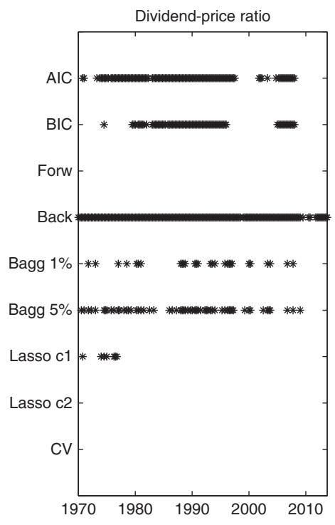
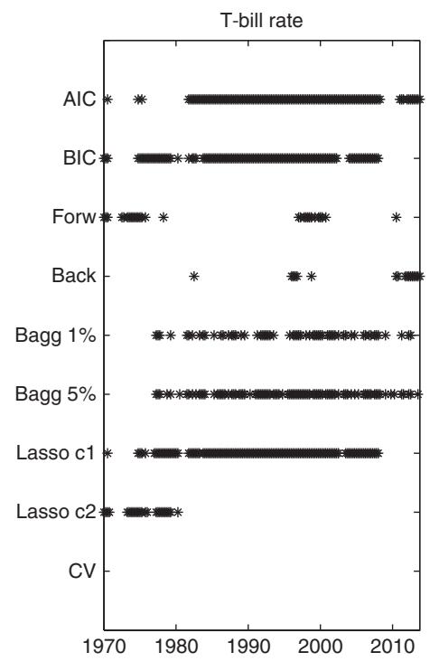
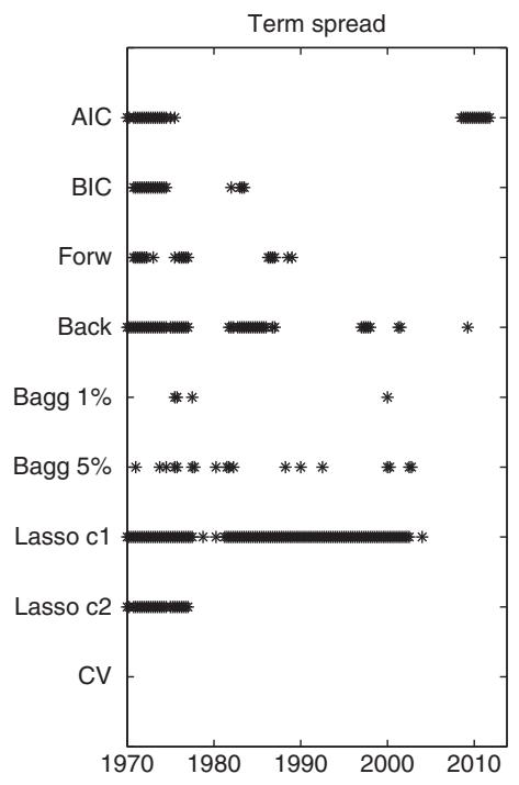
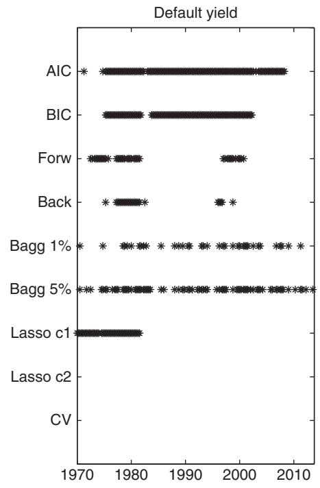
Figure 6.3: Recursive variable inclusion plots for the dividend–price ratio, the T-bill rate, the term spread, and the default yield in models fitted to quarterly US stock market returns. Variable inclusion is marked by an asterisk, while empty spaces indicate that the variable is not selected in a given period.
the opposite. The large negative values of the Diebold–Mariano test statistic obtained here indicate that the performance of the forecasts based on the AIC and BIC model selection criteria is particularly poor.
As argued previously, statistical measures of forecast performance are not necessarily closely aligned with economic measures of forecasting performance. To highlight this, we report two alternative measures of performance. First, we report the percentage of correctly predicted signs of excess returns or the “hit rate.” This is shown in column 6 of table 6.2. The numbers range between 51% for the models selected by the backward stepwise approach versus 61% for the prevailing mean and 60% for the Lasso method with the largest penalty term.
The highest hit rate is obtained simply by always predicting a positive mean excess return. This is a so-called “broken clock” forecast that never changes and therefore carries little or no information. A genuine ability to predict the sign of excess returns must entail some ability to forecast both positive and negative signs. The sign test proposed by Pesaran and Timmermann (1992), and explained in more detail in chapter 18, accounts for the forecasts’ ability to predict both positive and negative signs. Results for this test, which is asymptotically normally distributed, are shown in the seventh and eighth columns of table 6.2. These reveal no significant ability of any of the forecasting methods to pick models that correctly forecast the direction of the stock market.
练习题
What is the primary reason for studying out-of-sample results in forecasting models?
What is the maximum p-value used in the forward stepwise approach for a predictor to be added to the forecasting model?
In the Lasso method, what are the two values of used in the penalty factor formula?
Which of the following are true about the Bagging scheme implementation?
The cross-validation scheme discards 0.25t observations when constructing the estimation sample.
The prevailing mean forecast is less stable than other forecasts.
The backward stepwise approach uses a minimum p-value of ___ for a predictor to be removed from the existing model.
The formula for the penalty factor in the Lasso method is , where ___ for .
Explain how the Bagging scheme preserves dependence across observations.
What is the effect of increasing in the Bagging scheme on the selected model?
Which of the following statements are true regarding the time-series behavior of forecasts?
What is the primary advantage of studying out-of-sample results in forecasting models?
When implementing the Bagging scheme for forecasting, which of the following statements is correct regarding the treatment of autocorrelation in predictors?
Which of the following statements are true regarding the Lasso method for forecasting?
Explain how the choice of the penalty factor in the Lasso method affects the volatility of the forecasts, and relate this to the concept of shrinkage estimation.
登录后解锁笔记、知识点解析、AI 问答
立即登录