3.5 EMPIRICAL EXAMPLE: ASSET ALLOCATION WITH PARAMETER UNCERTAINTY

3.5 EMPIRICAL EXAMPLE: ASSET ALLOCATION WITH PARAMETER UNCERTAINTY

To illustrate and compare the use of classical and Bayesian prediction methods, consider the asset allocation problem of a buy-and-hold investor studied by Barberis (2000). There are two assets: T-bills and a stock market index. T-bills pay a constant, continuously compounded risk-free rate of $r_f$ . Suppose the continuously compounded excess return on stocks, ${\gamma }_t$ , is independently and identically distributed:

$$y_t=\mu +{\epsilon }_t,{\epsilon }_t\sim \mathrm{ind}\mathrm{N}(0,{\sigma }^2).\text{\hspace{1em}(3.31)}$$

Consider a buy-and-hold investor’s asset allocation decision at time T for an h-period investment horizon. Setting the investor’s initial wealth to $W_T=1$ and letting $\omega (z)$ be the allocation to the stock index, the investor’s terminal wealth at time $T+h$ is given by

$$W_{T+h}=(1-\omega (z))\exp (r_{f}h)+\omega (z)\exp \left(r_{f}h+\sum _{\tau =1}^h{y}_{T+\tau }\right).\text{\hspace{1em}(3.32)}$$

Suppose the investor has power utility over terminal wealth:

$$u(W_{T+h})=\frac{W_{T+h}^{1-A}}{1-A},\text{\hspace{1em}(3.33)}$$

where A is the coefficient of relative risk aversion. This utility function plays the role of the loss function with the difference that we seek to maximize expected utility rather than minimizing expected loss.

The investor chooses $\omega (z)$ as

$${\omega }^{\ast }(z)=\arg \underset{\omega (z)\in [0,1)}{\max }E\left[\frac{W_{T+h}^{1-A}}{1-A}|Z_T\right],\text{\hspace{1em}(3.34)}$$

where $E\left[.|Z_T\right]$ is the conditional expectation, given information at time $T,Z_T=$ $\{y_1,...,y_T\}$ . To rule out bankruptcy and unbounded expected utility, the weight on stocks is restricted to lie in [0, 1).

The classical and Bayesian methods differ in how they compute the expectation in (3.34). Under the classical plug-in approach, the investor conditions on the parameter estimates $\hat{\theta }=(\hat{\mu },{\hat{\sigma }}^2)$ and solves

$$\underset{\omega (z)\in [0,1)}{\max }\int \cdots \int u(W_{T+h}(\omega (z)){)}_{PY}(\sum _{\tau =1}^h{y}_{T+\tau }|Z_T,\hat{\theta })d{y}_{T+1}\dots d{y}_{T+h}.\text{\hspace{1em}(3.35)}$$

It follows from (3.31) that $\begin{array}{r}{p}_Y({\sum }_{\tau =1}^h{\gamma }_{T+\tau }|\hat{\theta },z_T)=\mathrm{N}(\hat{\mu }h,{\hat{\sigma }}^{2}h).\end{array}$ This solution ignores that $\theta$ is not known but typically estimated with considerable error.

The Bayesian approach deals with parameter uncertainty by integrating over the posterior distribution $p_Y(\theta |z_T)$ which summarizes the uncertainty about the parameters given the observed data sample $z_T$ . This leads to a predictive distribution which is conditioned only on the observed sample (and not on any estimate $\hat{\theta })$ :

$$\widehat{p_Y}(\sum _{\tau =1}^h{y}_{T+\tau }|Z_T)=\int d{p}_Y(\sum _{\tau =1}^h{y}_{T+\tau }|Z_T,\theta )\hat{p}(\theta |Z_T)d\theta .\text{\hspace{1em}(3.36)}$$

The Bayesian investor therefore solves

$$\begin{array}{rl}& \underset{\omega (z)\in [0,1)}{\max }\int \cdots \int u(W_{T+h}(\omega (z)))p_Y(\sum _{\tau =1}^h{y}_{T+\tau }|Z_T)d{y}_{T+1}\dots d{y}_{T+h}\\ & =\underset{\omega (z)\in [0,1)}{\max }\int \cdot \cdot \int u(W_{T+h}(\omega (z)))p_Y(\sum _{\tau =1}^h{y}_{T+\tau }|Z_T,\theta )p(\theta |Z)d{y}_{T+1}\dots d{y}_{T+h}d\theta .\end{array}\text{\hspace{1em}(3.37)}$$

This can be evaluated by sampling from the posterior distribution for ${\theta }_{:}$ , and, conditional on this draw, sampling from $p_Y({\sum }_{\tau =1}^h{y}_{T+\tau }|Z_T,\theta )$ , and finally averaging $u(W_{T+h})$ across those draws.

Barberis (2000) assumes an uninformative prior, $p(\mu ,{\sigma }^2)\propto {\sigma }^{-2}$ , and utilizes a normal-inverse gamma (IG) posterior distribution (see, e.g., Zellner (1971)),

$${\sigma }^2|Z_T\sim \mathrm{IG}(\frac{T-1}{2},\frac{1}{2}\sum _{t=1}^T(y_t-{\bar{y}}_T{)}^2),\text{\hspace{1em}(3.38)}$$

$$\mu |{\sigma }^2,Z_T\sim \mathrm{N}({\bar{y}}_T,\frac{{\sigma }^2}{T}),\text{\hspace{1em}(3.39)}$$

where ${\bar{y}}_T=(1/T){\sum }_{t=1}^T{y}_t$ is the sample mean. To solve for the optimal $\omega (z)$ Barberis considers a grid of values $\omega =0,0.01,0.02,\dots ,0.99$ and computes the integrals in (3.35) and (3.37) by numerical simulation. The idea is to draw a large number of (cumulated) returns $\{{\mathbf{y}}_{T+1:T+h}^i{\}}_{i=1}^I$ and then compute

$$\bar{U}(\omega (z))=\frac{1}{I}\sum _{i=1}^I\frac{{\left((1-\omega (z))\exp (r_{f}h)+\omega (z)\exp (r_{f}h+{\sum }_{\tau =1}^h{y}_{T+\tau }^i)\right)}^{1-A}}{1-A}.\text{\hspace{1em}(3.40)}$$

This calculation is straightforward in the classical case, given the assumption of normally distributed data: simply draw I times from $\mathrm{N}(\bar{\mu }h,{\hat{\sigma }}^{2}h);$ for each draw compute ${\sum }_{\tau =1}^h{y}_{T+\tau }$ , evaluate the utility function for a given value of $\omega (z)$ and average this across I . The value of $\omega (z)$ that yields the highest value of (3.40) is then the optimal allocation to stocks, ${\omega }^{\ast }(z)$

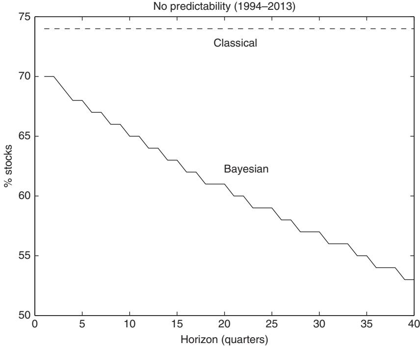
Figure 3.2: Optimal allocation to stocks under classical and Bayesian approaches.

To sample from the predictive distribution for long-horizon returns in the Bayesian case, $p_Y({\sum }_{\tau =1}^h{y}_{T+\tau }|Z_T)$ , first generate a sample $(\mu ,{\sigma }^2)$ from the posterior distribution for the parameters $p(\mu ,{\sigma }^2|Z_T)$ . Then sample from the distribution of long-horizon returns conditional on past data and the parameters, $\begin{array}{r}{p}_Y({\sum }_{\tau =1}^h{y}_{T+\tau }|\mu ,{\sigma }^2,Z_T)\end{array}$ . Finally, each of these draws is plugged into the utility function and averaged across the I draws to get an estimate of the average utility for a given value of ω(z).

Sampling from the posterior return distribution is very easy. First, we sample from the marginal distribution, $p({\sigma }^2|Z_T)$ , which by (3.38) is an inverse Gamma distribution. Given a value for ${\sigma }^2,$ , we next sample from the conditional distribution $p(\mu |{\sigma }^2,Z_T)$ which by (3.39) is a normal distribution. Finally, we sample from the distribution of returns conditional on the parameter values $\begin{array}{r}{p}_Y({\sum }_{\tau =1}^{h^{-}}{y}_{T+\tau }|\mu ,{\sigma }^2,Z_T)\end{array}$ . From (3.31) it follows that conditional on $(\mu ,{\sigma }^2)$ the cumulated return distribution is $\mathrm{N}(\mu h,{\sigma }^{2}h)$ .

Comparing the solutions in (3.35) and (3.37) gives a measure of the importance of parameter uncertainty for the investor’s optimal asset allocation. Figure 3.2 illustrates the difference in the percentage allocation to stocks (listed on the vertical axis) for the classical and Bayesian approaches for different investment horizons, h, measured in quarters and listed on the horizontal axis. The analysis uses quarterly returns data on a value-weighted portfolio of US stocks and a three-month T-bill rate over the 20-year period 1994Q1–2013Q4. The computations assume a coefficient of relative risk aversion of A = 5. The flat line shows the classical investor’s allocation to stocks.

This line is constant and so under i.i.d. returns the classical investor’s allocation to stocks is independent of the investment horizon. In contrast, the allocation to stocks under the Bayesian approach declines quite sharply from 70% at the 1-month horizon to around 55% at the 40-quarter (10-year) horizon.9

Such differences in asset allocations are a direct reflection of differences between how the classical and Bayesian approaches handle parameter uncertainty. Parameter uncertainty introduces another long-lasting source of risk; the true parameters could be worse than indicated by the sample, in which case long-run returns would be particularly adversely affected as the variance of the cumulative return distribution increases faster than linearly with the investment horizon, h. This leads risk-averse buy-and-hold investors to scale back their holdings of stocks and introduces horizon effects even under i.i.d. returns.