20.2.2 Long-Horizon Forecasts

20.2.2 Long-Horizon Forecasts

For stationary models with dynamic behavior that displays short memory, chapter 7 showed that the long-run forecast equals the unconditional mean of the variable. Thus, if we are interested in forecasting such variables far enough into the future, all we need to know about the variable is whether the dynamics have died out. For variables that are highly persistent, e.g., unit root processes, this conclusion is no longer true. For a model with a unit root, the long-run forecast is now the unconditional mean of the change in the variable plus the current observation and so the forecast depends on the present level of the data. For persistent variables, the model will have relevant information even at long horizons. As usual, we are most interested in forecasts conditional on the last observation.7 Unfortunately, results are not available for the very persistent models analyzed here, so we restrict ourselves to follow the literature and examine unconditional MSE loss.

Suppose the model for the data is given by (20.2) so the recursion in (20.3) remains relevant. Forecasts are constructed in the same way as for the short-horizon case discussed above, but now for large values of h. For purposes of the asymptotic theory, we typically take h to be large relative to the sample size T , such that $h=[\lambda T]$ ， where λ is the ratio of the forecast horizon to the sample size. Since h now diverges as the sample size becomes large, so does the unpredictable component ${\sum }_{i=1}^h{\rho }^{h-i}{\epsilon }_{T+i}$ in (20.3) and so the MSE diverges. However, rescaling the mean squared error by T results in a stable object that converges to a function of Brownian motions. The estimation error component in (20.3) also diverges at the same rate, so model estimation error is of the same order of magnitude as the unpredictable component, unlike in the short-horizon case. Analysis of the asymptotic properties of the MSE that use this approach to asymptotic theory, where $\rho$ is local to unity and $h=[\lambda T]$ has been undertaken by Stock (1996) and Phillips (1998), using a more general setup than here, and in Kemp (1999) and Turner (2004). These studies are reviewed by Elliott (2006).

To establish some results, let $h=\left[T\lambda \right]$ but now assume that estimation uses the first $T-h=T_1$ observations8 so we forecast ${\gamma }_T$ using observations $t=\{1,\dots ,T_1\}$ When the model is known, the forecast error scaled by $T^{-1/2}$ is

$$\begin{array}{rl}{T}^{-1/2}{\sum }_{i=1}^h{\rho }^{h-i}{\epsilon }_{T_1+i}=T^{-1/2}(y_{T_1+[T\lambda ]}-{\rho }^h{y}_{T_1})& \\ & =T^{-1/2}(y_T-{\rho }^h{y}_{T_1})\\ & \Rightarrow {\sigma }_{\epsilon }\{M(1)-e^{-\gamma \lambda }M(1-\lambda )\}.\end{array}$$

Hence, the long-horizon forecast diverges, as we might expect since $h$ is diverging. The expectation of the square of this limit is ${\sigma }_{\epsilon }^2(1-{\bar{e}}^{-2\gamma \lambda })\overline{/}(2\gamma )$ when $\rho <1$ and is independent9 of the initial condition, α. In the presence of a unit root, the mean of the squared forecast error divided by $T$ equals $\lambda {\sigma }_{\epsilon }^2$

Suppose, alternatively, that we impose a unit root. When $d_t=1$ this means that we use ${\gamma }_{T_1}$ to forecast ${\gamma }_T$ . The scaled forecast error is now

$$T^{-1/2}(y_T-y_{T_1})\Rightarrow {\sigma }_{\epsilon }\{M(1)-M(1-\lambda )\}.$$

The expectation of this term is

$$\frac{1-e^{-\gamma \lambda }}{\gamma }+\frac{({\alpha }^2-1)e^{-2\gamma }(1-e^{\gamma \lambda }{)}^2}{2\gamma }.\text{\hspace{1em}(20.6)}$$

The estimation error and the unpredictable component are now of the same order, unlike in the fixed horizon case. For $\rho <1$ , the expectation in (20.6) is greater than that for the known model. When $d_t=(1,t)$ , the additional terms due to model misspecification error are

$$T^{-1/2}(y_T-y_{T_1}-{\hat{\varphi }}_{2}h)\Rightarrow {\sigma }_{\epsilon }(M(1)-M(1-\lambda )-\lambda (M(1-\lambda )-M(0))).$$

The mean of the square of this term is lengthy and not particularly informative.

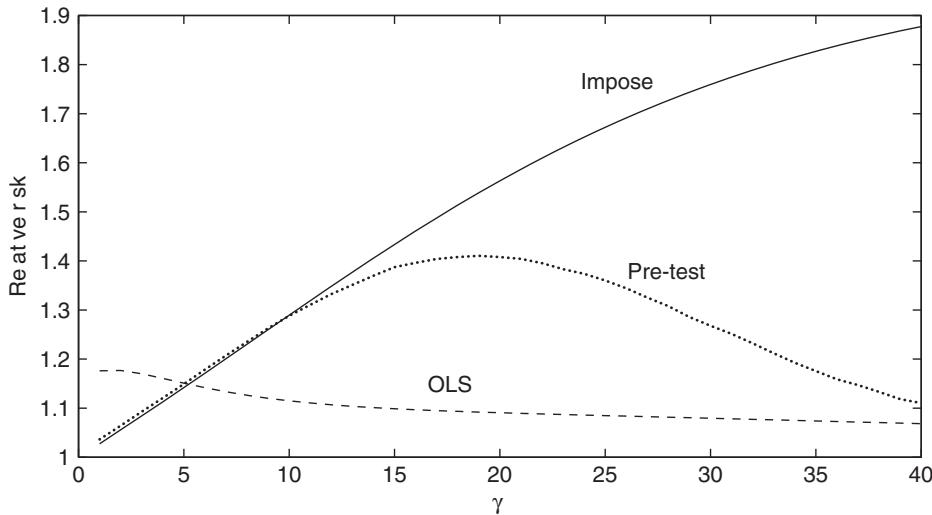
Figure 20.3: Long-horizon risk under three different approaches. The figure plots the risk component b as a function of the local-to-unity parameter $\gamma$ for three different approaches: (i) imposing a unit root (full line); (ii) estimating the model parameters (dash-dotted line); (iii) pre-testing for a unit root (dotted line). The figure assumes a long forecast horizon of $\lambda =0.1$ , i.e., 10% of the full sample and includes a constant deterministic term.

Estimation of the model parameters results in the expressions becoming even more abstract, although they have been given in Stock (1996), Phillips (1998), and Turner (2004). Rather than state the results, we note that estimation error is again of the same order as the unpredictable component, similar to what we found when imposing the unit root. To visualize the results, we examine the trade-offs of the same methods examined for short horizons but now for much longer horizons up to $h=40$ periods.

Figure 20.3 shows the risk for the three approaches—imposing a unit root, estimating the model parameters, or the hybrid approach based on a pre-test— measured relative to the infeasible risk under the known model. The first panel assumes $d_t=1$ , while the second is for $d_t=(1,t{)}^{\prime }$ . Each panel assumes $\lambda =0.1$ . The basic results are similar to the situation with a fixed horizon, namely that imposing a unit root works well if this is close to being the correct model. However, this approach quickly gets overwhelmed by simply estimating the parameters. Pre-testing does not really provide a useful way to combine the good properties of imposing the root when the root is close to 1 and estimating it when the root is far from 1, because the pre-test method (as seen in the stationary case) does not have the power to clearly distinguish between the two choices in the region where such a distinction becomes useful.

The main difference compared with the stationary case is that the cutoff point where imposing a unit root versus estimating it works equally well is now larger and occurs for values of $\gamma$ further away from 1. The need to estimate the contribution of the trend component seems to further increase the cutoff value.

Because the distributions above depend on the unknown value of $\gamma ,$ , it is difficult to construct confidence intervals for ${\gamma }_T$ given the data $\{y_1,\dots ,y_{T_1}\}$ . When $\gamma =0$ so there is an exact unit root,

$$T^{-1/2}(y_T-y_{T_1})\Rightarrow {\sigma }_{\epsilon }^2\left\{W(1)-W(1-\lambda )\right\}=\mathrm{N}(0,\lambda {\sigma }_{\epsilon }^2).$$

In this case it makes sense to construct confidence intervals using $y_T\stackrel{a}{\sim }\mathrm{N}(y_{T_1},h{\sigma }_{\epsilon }^2)$ so that a $(1-\alpha )\%$ confidence interval for ${\gamma }_T$ $\{y_{T_1}\pm c{v}_{\alpha }\sqrt{h}{\sigma }_{\epsilon }^2\}$ , where $c{v}_{\alpha }$ is the α% critical value. In the general case, however, the distribution of the forecast error obtained either by imposing a unit root or by estimating the root will depend on $\gamma$ (and potentially α). There are no currently available methods to deal with this dependence.