17.6 ADDRESSING DATA MINING

17.6 ADDRESSING DATA MINING

White’s Reality Check provides a way to address a question that arises when selecting which variables, $z_t.$ , to include in the orthogonality regression. The vast array of possible covariates along with the wide set of choices of models means that one can search over many possible specifications. Indeed, this is exactly how the literature has proceeded with different researchers using different forecasting models. Suppose that a researcher finds a superior model. How should we interpret this evidence if the model were preceded by numerous other specifications? One way is to consider the model as the (potentially) best model among a larger set of competing specifications and use White’s Reality Check approach to correct for the effect of the search across multiple models. In other words, we would examine whether the best of the specifications really does outperform the baseline, taking into account the other models that were tried out. This is the approach taken by Sullivan, Timmermann, and White (2001) to study the performance of technical trading rules applied to daily stock returns.

An alternative to the White–Hansen approach is to use a Bonferroni bound. Let $p_k$ be the p-value associated with the null that model k does not produce lower expected loss than the benchmark. For arbitrary correlations between the performance measures, ${\bar{d}}_1,\dots ,{\bar{d}}_m,$ the Bonferroni bound implies that the $p\cdot$ -value for the joint null that none of the m models is superior to the benchmark satisfies an upper bound,

$$\begin{array}{r}p\le \min (m\times \min (p_1,...,p_m),1).\end{array}\text{\hspace{1em}(17.43)}$$

Equivalently, the test rejects at the α% critical level if min $(p_1,...,p_m)<\alpha /m$ . Note that the smallest of the p-values, which produces the strongest evidence against the null that no model beats the benchmark, gets multiplied by the number of models under consideration. The Bonferroni approach tends to be conservative and guards against “worst case” scenarios. For example, in the case of perfectly correlated forecasts, the p-values are identical and so the correct procedure is to reject if $\mathbf{p}<\alpha$ rather than rejecting only for $p<\alpha /m$

Both equations (17.42) and (17.43) illustrate that, from the perspective of being able to identify a truly superior model, it is not innocuous to search across a large set of prediction models, many of which have no hope of producing good results. Every time a new alternative model is considered, the yardstick for beating the benchmark gets adjusted, thereby imposing a “tax” on mindless data mining efforts. Procedures that can direct the search for a forecasting model by using economic theory to identify either functional form or predictor variables, therefore have a better hope of being successful.

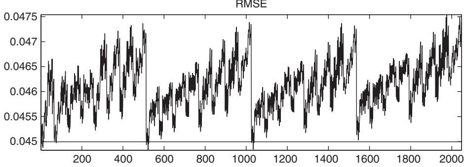
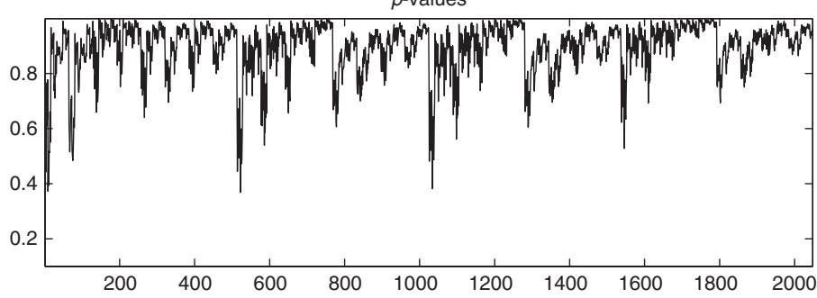
Figure 17.1: Root mean squared error performance (top) and p-value (bottom) measured against the prevailing mean benchmark and based on all possible combinations of 11 predictor variables. All forecasts are based on estimates using a rolling window with 20 years of monthly observations.

17.6.1 Empirical Application

To illustrate these ideas, we undertook an empirical application to monthly stock returns using the 11 predictor variables from the Welch and Goyal (2008) data set included in the earlier application. We consider all possible $2^{11}=2048$ models. The out-of-sample period is 1970–2013 and estimates are updated using a rolling estimation window with 20 years of monthly observations. This ensures that nested models do not become an issue when applying White’s Reality Check or Hansen’s SPA test. We use the prevailing mean model of Welch and Goyal (2008) as our benchmark. This includes an intercept but no time-varying predictors.

The top panel in figure 17.1 plots the RMSE performance with the value for the benchmark prevailing mean model shown as a horizontal line. The patterns in the plots reflect the ordering of the models which is not random but has small models followed by larger models within different blocks comprising the different predictors. Very few models manage to produce a lower RMSE performance than the prevailing mean benchmark.

The bottom panel in figure 17.1 plots the p-values associated with the individual models. None of the models appear able to generate p-values close to the conventional 5% cutoff. Thus it is not surprising for this application that none of the models beat the prevailing mean benchmark after accounting for model search. In fact, when we use White’s Reality Check, this yields a p-value of 1, confirming that the best forecasting model does not outperform the prevailing mean benchmark.