15.2 LOSS DECOMPOSITION METHODS

15.2 LOSS DECOMPOSITION METHODS

Methods for decomposing the loss are popular in the applied forecasting literature, particularly under squared error loss. Theil (1961) suggested the following decomposition:

$$\begin{array}{rl}E[y-f{]}^2=E[(y-Ey)-(f-Ef)+(Ey-Ef){]}^2& \\ & \\ & =E[y-Ey{]}^2+E[f-E(f){]}^2+(Ey-Ef{)}^2\\ & \\ & -2E[(y-Ey)(f-Ef)]\end{array}$$

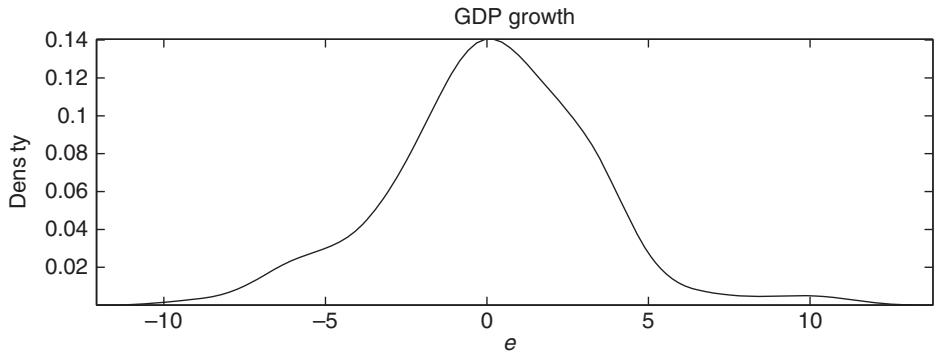
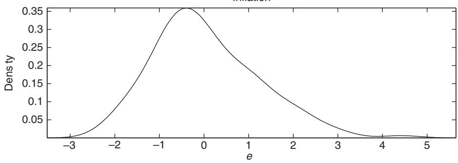
Figure 15.5: Density plots for the one-quarter-ahead forecast errors from the Federal Reserve’s Greenbook forecasts of GDP growth and the inflation rate.

$$\begin{array}{rl}& =(Ey-Ef{)}^2+{\left(\sqrt{E[y-Ey{]}^2}-\sqrt{E[f-E(f){]}^2}\right)}^2\\ & +2\sqrt{E[y-Ey{]}^2}\sqrt{E[f-E(f){]}^2}(1-\rho )\\ & =(Ey-Ef{)}^2+({\sigma }_y-{\sigma }_f{)}^2+2{\sigma }_y{\sigma }_f(1-\rho ),\end{array}\text{\hspace{1em}(15.1)}$$

where $\rho ={\sigma }_{yf}/({\sigma }_f{\sigma }_y)$ is the correlation between y and $f{.}^1$ The sample analog to this expression is

$$\begin{array}{c}\frac{1}{T-h}\sum _{t=1}^{T-h}(y_{t+h}-f_{t+h|t}{)}^2=\frac{1}{T-h}\sum _{t=1}^{T-h}((y_{t+h}-\bar{y})-(f_{t+h|t}-\bar{f})+(\bar{y}-\bar{f}){)}^2\\ ={\hat{\sigma }}_y^2+{\hat{\sigma }}_f^2+(\bar{y}-\bar{f}{)}^2-2{\hat{\sigma }}_{yf}\\ =(\bar{y}-\bar{f}{)}^2+({\hat{\sigma }}_y-{\hat{\sigma }}_f{)}^2+2({\hat{\sigma }}_y{\hat{\sigma }}_f-{\hat{\sigma }}_{yf})\\ =(\bar{y}-\bar{f}{)}^2+({\hat{\sigma }}_y-{\hat{\sigma }}_f{)}^2+2{\hat{\sigma }}_y{\hat{\sigma }}_f(1-\hat{\rho }).\end{array}\text{\hspace{1em}(.2)}$$

Here $\begin{array}{r}\bar{y}=(T-h{)}^{-1}{\sum }_{t=1}^{T-h}{y}_{t+h}\end{array}$ and $\bar{f}=(T-h{)}^{-1}{\sum }_{t=1}^{T-h}{f}_{t+h|t}$ are sample means and $\hat{\rho }={\hat{\sigma }}_{yf}/({\hat{\sigma }}_y{\hat{\sigma }}_f)$ , where ${\hat{\sigma }}_y,{\hat{\sigma }}_f,{\hat{\sigma }}_{yf}$ are sample estimates of ${\sigma }_y,{\sigma }_f$ , and Cov(y, f ), respectively.

The first term in (15.2) measures the difference in the means of the forecast and outcome and so captures whether the average forecast is close to the average outcome. This term is 0 when the average outcome and forecast lie on the $45^{\circ }$ line in the scatterplot of forecasts versus outcomes. A large value of this term indicates that average forecasts are off center, or biased. For forecasts constructed using lagged values of the outcome, this term is unlikely to be large.

The second term in (15.2) measures differences between the standard deviations of $f$ and y and captures whether the variation in the forecasts is similar to that of the outcomes. For hard-to-predict variables such as stock returns, this term tends to be very large since the fluctuation in the outcome is an order of magnitude greater than that of the forecasts. Conversely, if forecasts are generated by a random walk model that sets $f_{t+h|t}=y_t$ , this term will be close to 0 since the forecast and outcome display the same amount of variability.

The last term in (15.2) depends on the correlation between the forecast and the outcome and is smaller, the larger their correlation. This term will be large for hardto-predict variables, although the scaling by ${\hat{\sigma }}_f$ may reduce this term.

An alternative approach, more commonly seen in binary prediction for which it was originally developed, decomposes mean squared errors into calibration and resolution terms:

$$\begin{array}{rl}& E[y-f{]}^2=E[(y-E[y])-(f-E[y|f])-(E[y|f]-E[y]){]}^2\\ & =E[(y-E[y]{)}^2]+E[(f-E[y|f]{)}^2]+E\left[(E[y|f]-E[y]{)}^2\right]\\ & -2E[(y-E[y])(E[y|f]-E[y])]+2E[(f-E[y|f])(E[y|f]-y)]\\ & -2E[(y-E[y])(f-E[y|f])]\\ & =E\left[(y-E[y]{)}^2\right]+E\left[(f-E[y|f]{)}^2\right]-E\left[(E[y|f]-E[y]{)}^2\right].\end{array}\text{\hspace{1em}(15.3)}$$

Here unconditional expectations are taken over both y and $f.$ The first term in this decomposition is the unconditional variance of the outcome variable. This does not depend on the forecast and so can be taken as given for the remainder of the analysis. Calibration is defined as $E[y-f|f]$ . For any forecast, $f,$ , this measures the difference between the expected value of the outcome given the forecast and the forecast itself. Hence, the second term in (15.3) equals the average squared calibration error, where the average is taken over f. A well-calibrated model has a calibration measure of 0 for all $f.$ .

The last term in (15.3) is known as the resolution term and enters with a minus sign. Resolution measures the squared average (computed over all forecasts) of the difference between the average outcome conditional on the forecast and the unconditional average outcome. This term will be small, indicating poor resolution, if, conditional on the forecast, the average value of the outcome is equal to the unconditional average value of the outcome for a wide range of forecasts. In such cases, the forecast is not picking up much variation in the outcome variable apart from its mean. Conversely, high resolution is achieved when the forecast picks up a lot of the variation in the outcome variable and $E\left[\mathbf{y}|\mathbf{f}\right]-E\left[\mathbf{y}\right]$ tends to be large.

Estimation of the terms in the decomposition in (15.3) requires estimates of the distribution of the outcome variable conditional on the forecast. A common approach is to discretize the forecast to enable such calculations. Galbraith and van Norden (2011) propose to use nonparametric methods for the case with continuous forecasts.

The decomposition can be modified for data that appear nonstationary or show trending behavior by setting $\begin{array}{r}(T-h{)}^{-1}{\sum }_{t=1}^{T-h}(y_{t+h}-f_t{)}^{-}=(T-h{)}^{-1}{\sum }_{t=1}^{T-h}([y_{t+h}-\end{array}$ $y_t]-[{\bar{f}}_t-y_t]{)}^2$ . The interpretation of the various components in the decompositions now applies to the actual and predicted change. This ensures that the variance and covariance terms can be estimated consistently when samples become large and is similar to first-differencing data to induce stationarity for variables with a unit root.

An important limitation of these decompositions is that there are no objective measures for how large or small the terms should be for any particular forecasting problem. Moreover, the terms are typically correlated so that one model’s improvement in a specific term may result in a deterioration in the other terms. In this case, a reasonable forecast improvement would require that the improvement in one of the terms more than offsets any reductions in performance in the other terms.