正在学习
14.4.2 Empirical Illustration
14.4.2 Empirical Illustration
To illustrate the various model combination approaches, we study monthly growth in the industrial production index, log(IPt). We consider three univariate and one multivariate approach to forecasting this variable, namely (AR) models (described in chapter 7); artificial neural net (ANN) models (chapter 11); and smooth threshold autoregressive (STAR) models (chapter 8), all with lag length selected by the AIC— and multivariate dynamic factor models (chapter 10). We first consider which of these models gets selected based on past MSE performance. This will of course vary with the length of the evaluation window, so we consider both 5- and 10-year windows. Our estimation sample runs from 1948:01 to 1969:12, which leaves the period 1970:01–2010:12 for out-of-sample forecast evaluation.
Figure 14.9 presents the results. If one model were dominant, we would expect it to get selected in most periods, barring random variation. This is not what we find. In fact, the dynamic factor model seems to dominate in the earliest part of the sample, followed by a period where the AR model performs best under the 5-year evaluation window method, while the STAR model is best under the 10-year evaluation window.
5 years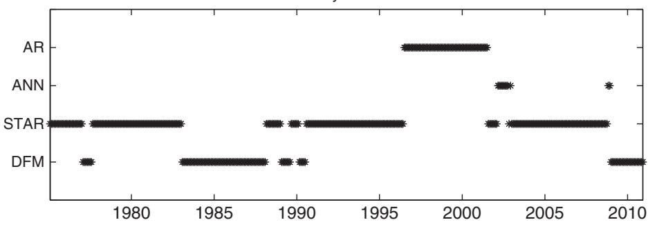
10 years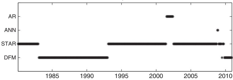
Figure 14.9: Best forecasting method for monthly growth in industrial production based on the root mean squared forecast error calculated over a rolling 5-year window (top) or a rolling 10-year window (bottom) for autoregressive (AR), artificial neural net (ANN), smooth threshold autoregression (STAR), and dynamic factor (DFM) models.
Figure 14.10 shows how the OLS estimates of the combination weights on STAR and DFM forecasts evolve over time. The weights show considerable variation over time, with the weight on the STAR forecasts being particularly volatile, and differ sharply from the value of 0.25 implied by equal weighting across the four forecasting methods.
How sensitive are the forecasts to using different weighting schemes? To address this issue, figure 14.11 plots time series of forecasts from combinations that use equal weights (top), OLS weights (second), inverse MSE weights (third), and the previous best model (bottom). The forecasts are quite similar but also show notable differences with the OLS weights leading to the greatest range of forecast variation. The similarities in performance across different combination schemes indicate that there are not great gains to be had by using the more complicated combination schemes such as OLS weighting or inverse MSE weighting compared with simply using equal weights.
Table 14.1 reports out-of-sample forecasting performance for the various forecast combination schemes in addition to the previous best model and the performance of the individual models. The left column reports RMSE values, while the right column shows values for the Diebold–Mariano test statistic, computed relative to the equal-weighted combination forecast which is thus the benchmark. Positive values are indicative that a method generates more accurate forecasts than this benchmark, while negative values suggest the opposite. The results confirm the impression from figure 14.11. Indeed, the equal-weighted combination produces the second lowest RMSE value after the inverse MSE weighting and the two approaches differ only by a small margin.
5 years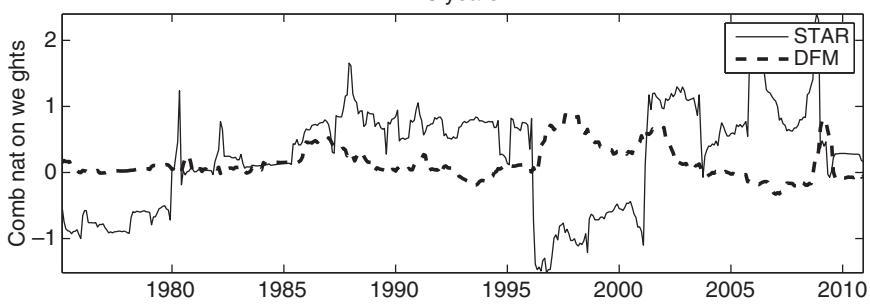
10 years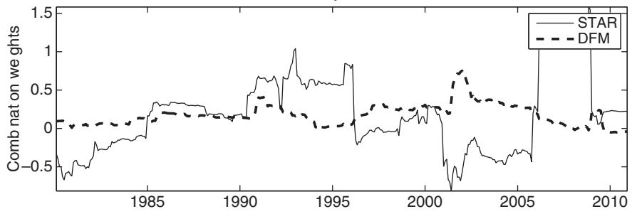
Figure 14.10: Estimated forecast combination weights on autoregressive (AR), artificial neural net (ANN), smooth threshold autoregression (STAR), and dynamic factor (DFM) models using rolling 5-year (top) and rolling 10-year (bottom) estimation windows applied to monthly growth in industrial production.
Equal weights
OLS weights
Inverse MSE weights
Best model
Figure 14.11: Combined forecasts using equal weights (EW), recursively estimated least squares weights (OLS), inverse MSE weights (MSE), and the previous best forecast method applied to the monthly growth in industrial production.
TABLE 14.1:
Root mean squared errors for out-of-sample forecasts of the monthly growth in industrial production based on rolling 10-year estimation windows. The top panel shows results for different combination methods, while the bottom panel shows results for the individual forecasting models with lag length selected by the AIC.
| Method | RMSE | DM stats |
| EW | 0.6685 | 0.0000 |
| Previous best | 0.7113 | -1.4885 |
| Inverse MSE | 0.6672 | 0.3949 |
| OLS | 0.6933 | -1.4792 |
| AR | 0.6720 | -0.3420 |
| ANN | 0.6761 | -0.5845 |
| STAR | 0.6972 | -1.5199 |
| DFM | 0.8315 | -3.4361 |
Selecting the single model with the previous best forecast performance appears to be a bad forecasting strategy. It is also of interest to compare the combination approach to the performance of the individual models. From the bottom part of table 14.1 it is clear that the best combination strategy always performs better than the best individual model. This is again an argument for combining models, rather than attempting to select a single best model.
练习题
Which model performed best under the 5-year evaluation window during the middle period of the sample?
What was the estimation sample period for the industrial production index forecasting study?
Which models were considered for forecasting the monthly growth in the industrial production index?
Which of the following statements about combination weights are true?
The equal-weighted combination produces the lowest RMSE value compared to all other combination schemes.
Selecting the single model with the previous best forecast performance is a good forecasting strategy.
The best combination strategy always performs better than the best ___.
The ___ model seems to dominate in the earliest part of the sample.
Explain why the forecasts are quite similar but also show notable differences with the OLS weights leading to the greatest range of forecast variation.
What is the Diebold–Mariano test statistic used for, and what do positive and negative values indicate?
When evaluating forecasting models for monthly growth in industrial production using a 5-year window, which model performed best according to the empirical illustration?
Which of the following statements are true regarding the combination weights over time for forecasting industrial production growth?
The equal-weighted combination of forecasts generally produces lower RMSE values compared to more complicated combination schemes such as OLS weighting or inverse MSE weighting.
The ___ method of combining forecasts involves assigning weights based on the inverse of the estimated variance of the forecast error, adjusted so that the weights sum to 1.
Explain why selecting the single best model based on previous best forecast performance might be a bad strategy.
登录后解锁笔记、知识点解析、AI 问答
立即登录