14.4.1 Complete Subset Regressions

14.4.1 Complete Subset Regressions

Elliott, Gargano, and Timmermann (2013) propose an estimation method that uses equal-weighted combinations of forecasts based on all possible models restricted to include a fixed (given) number of regressors, $k\le K$ . The approach, which they name complete subset regressions, first regresses the outcome, ${\mathbf{\gamma }}_t,$ on a given subset of the regressors, then averages the results across all k-dimensional subsets of the regressors.

Assuming K regressors in the full model and k regressors chosen for each of the subset models, there will be $n_{k,K}=K!/(k!(K-k)!)$ subset regressions to average over. For example, the univariate case, $k=1$ , yields $n_{1,K}=K$ regressions, each of which includes a single variable. All elements of ${\hat{\mathbf{\beta }}}_i$ are 0 except for the least squares estimate of $y$ on $x_i$ in the ith row. The equal-weighted combination of forecasts from the individual univariate regression models becomes

$$f^c=\frac{1}{K}\sum _{i=1}^K{x}_i^{\prime }{\hat{\beta }}_i.\text{\hspace{1em}(14.25)}$$

Subset regression coefficients can be computed as averages over least squares estimates of the subset regressions. When the covariates are correlated, the individual regressions will be affected by omitted variable bias, but Elliott, Gargano, and

Timmermann (2013) show that the subset regression estimators are themselves approximately a weighted average of the full regression OLS estimator, ${\hat{\mathbf{\beta }}}_{\mathrm{ols}}$ . Assume that K is fixed and let $S_i$ be a $(K\times K)$ matrix with 0s everywhere except for 1s in the diagonal cells corresponding to included variables, so that if the $(j,j)$ element of $S_i$ is 1, the j th regressor is included, while if this element is 0, the j th regressor is excluded.

Provided that as the sample size gets large, ${\hat{\mathbf{\beta }}}_{\mathrm{ols}}\to \mathbf{P}{\beta }_0$ for some ${\beta }_0$ and $T^{-1}{X}^{\prime }X{\to }^p{\Sigma }_X$ , the estimator for the complete subset regression, ${\hat{\beta }}_{k,K}$ , can be written as

$${\hat{\beta }}_{k,K}={\Lambda }_{k,K}{\hat{\beta }}_{\mathrm{ols}}+o_P(1),\text{\hspace{1em}(14.26)}$$

where

$${\Lambda }_{k,K}\equiv \frac{1}{n_{k,K}}\sum _{i=1}^{n_{k,K}}{\left(S_i^{\prime }{\Sigma }_X{S}_i\right)}^{-}(S_i^{\prime }{\Sigma }_X).$$

In the special case where the covariates are orthonormal and ${\hat{\beta }}_{k,K}={\lambda }_{k,K}{\hat{\beta }}_{\mathrm{ols}}$ with ${\lambda }_{k,K}=1-(n_{k,K-1}/n_{k,K})$ being a scalar, subset regression reduces to Ridge regression.

The amount of shrinkage implied by ${\lambda }_{k,K}$ depends on both k and K and the smaller is k relative to $K_i$ , the greater the amount of shrinkage. This result relates shrinkage provided by model averaging to shrinkage on the individual coefficients whereas a typical Bayesian approach would separate the two. In general ${\Lambda }_{k,K}$ reduces to the Ridge estimator, either approximately or exactly, only if the regressors are uncorrelated. If this does not hold, subset regression coefficients cannot be interpreted as the outcome of simple regressor-by-regressor shrinkage of the OLS estimates, and instead depend on the full covariance matrix of all regressors.

Figure 14.8 illustrates the complete subset regression approach for our earlier application to US stock returns. We use a list of 11 possible predictor variables, so $K=11$ in this application. Along the horizontal axis we plot k, the number of included predictors which varies from $k=0$ (the prevailing mean) to $k=11$ (kitchen sink model). The root mean squared error is plotted on the vertical axis. For each value of k, the column of circles shows the RMSE values of all models with exactly k predictors, whereas the solid triangle shows the average RMSE value computed across these models. For example, there are 11 different RMSE values for $k=1$ and for $k=10$ , and 55 different RMSE values for $k=2$ and for $k=9$ . The range of values is larger in the middle, reflecting in part the bigger set of models being compared for these middle values of k. Note, however, that the average RMSE performance for a given value of k is trending upwards as k grows larger. This reflects the increased importance of estimation error for larger sets of regressors.

The curved line underneath the circles gives the RMSE value for the complete subset regressions corresponding to a given value of k. Notably, this line is lower than the lowest RMSE value of any individual model with the same number of regressors. The minimum value of the complete subset regression line is reached for $k=2$ . At this point (as well as for $k=1\mathrm{or}k=3)$ , the RMSE of the complete subset regression forecast is lower than that of the prevailing mean. It is also lower than the RMSE associated with the equal-weighted average forecast computed across all models, which tends to put too much weight on models with large numbers of regressors and poor forecasting performance.

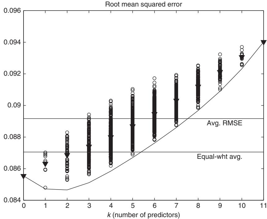
Figure 14.8: Complete subset regression combination forecasts of stock returns using 11 predictors.

In settings with large-dimensional sets of predictors with weak power, Elliott, Gargano, and Timmermann (2015) show analytically that the complete subset regression approach achieves variance reduction and find empirically in applications to US unemployment, GDP growth, and inflation (as well as in Monte Carlo simulations) that the approach establishes a more favorable bias–variance trade-off than univariate models or dynamic factor models.