13.4.1.2 Mixtures of Normals

13.4.1.2 Mixtures of Normals

Mixtures of normals assume that $y_{t+1}$ is a mixture of Gaussian components:

$$y_{t+1}={\mu }_{s_{t+1}}+{\sigma }_{s_{t+1}}{\eta }_{t+1},{\eta }_{t+1}\sim \mathrm{ind}\mathrm{N}(0,1),\text{\hspace{1em}(13.32)}$$

where ${\mu }_{s_{t+1}}$ is the mean conditional on being in state $s_{t+1}$ while ${\sigma }_{s_{t+1}}$ is the volatility in state $s_{t+1}$ . The state variable, $S_{t+1}$ , takes a finite number of values, $S_{t+1}\in \{1,\dots ,K\}$ and is typically assumed to be generated by a first-order homogeneous Markov chain:

$$\mathrm{Pr}(s_{t+1}=i|s_t=j)=p_{ij}.\text{\hspace{1em}(13.33)}$$

Note the crucial distinction between a weighted sum of normally distributed variables, which will be normally distributed, and a mixture of normal distributions. Mixtures of Gaussian distributions are not Gaussian. Instead, they resemble compound lotteries: first nature draws a state $s_{t+1}$ , then it draws an outcome from the resulting state distribution. Only one of the states occurs at each point in time, but it is not known ahead of time which one will occur. This property can be used to create a flexible set of density forecasts.

TABLE 13.2:
Estimates of two-state Markov switching fitted to daily US stock market returns (1990–2015).

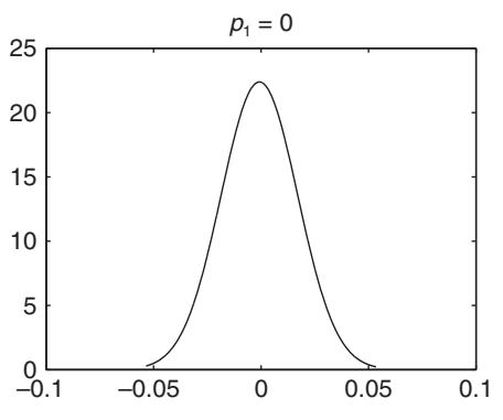
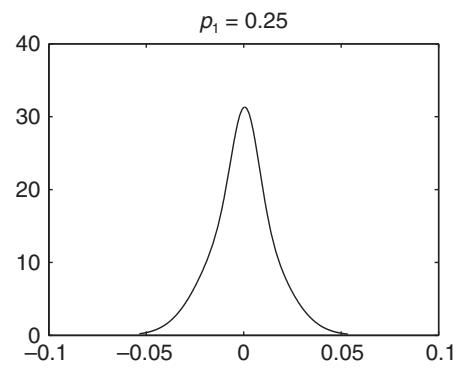
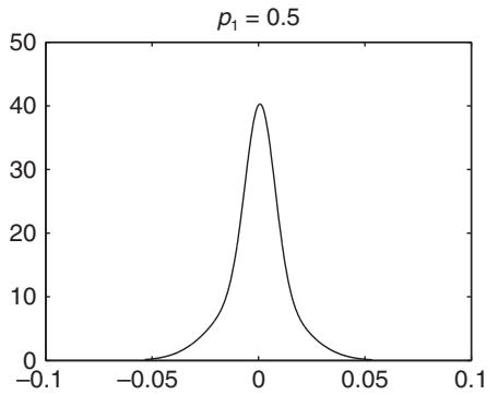
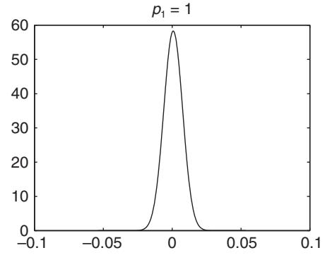
Figure 13.5: Density plots for the two-state Markov switching process fitted to daily US stock market returns, using four different probability weights for the two states.

We next estimate a two-state Markov switching model on daily US stock returns over the period 1990–2010, i.e., the same data used to generate the volatility plot in figure 13.1. The parameter estimates for this model are shown in table 13.2; the estimates indicate that state two is a low-mean, high-volatility regime, while state one is a high-mean, low-volatility state. As revealed by the state transition probabilities, both states are highly persistent although the high-mean, low-volatility state is notably more persistent $({\hat{p}}_{11}=0.988)$ than the low-mean, high-volatility state $({\hat{p}}_{22}=0.971)$ .

Figure 13.5 shows the density implied by this model for four different values of the probability of state one, namely $p_1=\{0,0.25,0.5,1\}$ . When $p_1=0\mathrm{or}{p}_1=1$ the densities are Gaussian and differ only because the standard deviation is much higher in state two than in state one. However, when $p_1=0.25$ or $\begin{array}{r}{p}_1=\mathrm{0.5.}\end{array}$ , there is clear evidence of kurtosis, with a more peaked distribution and a slower tail decay than under the normal distribution.

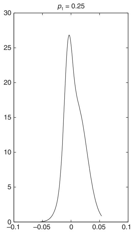
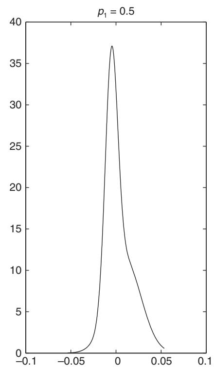
Figure 13.6: Density plots for the Markov switching process with ${\mu }_1=-0.5\%$ and ${\mu }_2=1\%$ and volatility parameters as in figure 13.5.

To further highlight this point, figure 13.6 plots two mixture distributions for $p_1=0.25$ and $p_1=0.5$ , using the same volatility parameters as in the previous plot, but setting ${\mu }_1=-0.5\%$ and ${\mu }_2=1\%$ . Using these more extreme differences in mean parameters, we clearly see how the two-state mixture distribution is right skewed.

In fact, the density of a mixture is a weighted average of the individual densities, with weights that represent the probability of being in the respective states conditional on current information:

$$p_Y(y_{t+1}|Z_t)=\sum _{j=1}^K{p}_Y(y_{t+1}|s_{t+1}=j,Z_t)P(s_{t+1}=j|Z_t).\text{\hspace{1em}(13.34)}$$

Given the state transition probabilities in (13.33) the conditional state probabilities can be derived from the total probability theorem:

$$\mathrm{Pr}(s_{t+1}=j|Z_t)=\sum _{j=1}^K{p}_{ij}P(s_t=i|Z_t).\text{\hspace{1em}(13.35)}$$

Moments of mixture distributions are easily derived. For example, the centered unconditional moments of the Markov switching process (13.32)–(13.33) are given by

$$E\left[(y_{t+1}-\mu {)}^n\right]=\sum _{i=1}^K{\pi }_i\sum _{j=0}^n{}_n{C}_j{\sigma }_i^{j}E[{\eta }_t^j]({\mu }_i-\mu {)}^{n-j},\text{\hspace{1em}(13.36)}$$

where ${}_n{C}_j=n!/((n-j)!j!)$ and ${\pi }_i$ is the steady-state probability of being in state $i;$ see Timmermann (2000).

Suppose $k=2$ so that there are two states and assume that the innovations, η, are normally distributed. Then the steady state probabilities are given by

$${\pi }_1=\frac{1-p_{22}}{2-p_{11}-p_{22}},{\pi }_2=\frac{1-p_{11}}{2-p_{11}-p_{22}}.\text{\hspace{1em}(13.37)}$$

The unconditional mean and variance of y take the forms

$$\begin{array}{l}\mu ={\pi }_1{\mu }_1+{\pi }_2{\mu }_2,\\ {\sigma }^2={\pi }_1{\sigma }_1^2+(1-{\pi }_1){\sigma }_2^2+(1-{\pi }_1){\pi }_1({\mu }_2-{\mu }_1{)}^2.\end{array}$$

This is not simply a weighted average of ${\sigma }_1^2$ and ${\sigma }_2^2$ and also depends on the difference in means $({\mu }_1-{\mu }_2{)}^2$

Similarly, the centered skew is given by

$$\begin{array}{rl}& \mathrm{skew}=E\left[(y-\mu {)}^3\right]\\ & ={\pi }_1(1-{\pi }_1)({\mu }_1-{\mu }_2)\left\{3({\sigma }_1^2-{\sigma }_2^2)+(1-2{\pi }_1)({\mu }_2-{\mu }_1^2{)}^2\right\}.\end{array}$$

For this to be nonzero requires that ${\mu }_1\ne {\mu }_2$

Conditional moments can be derived by using conditional state probabilities $p_{1t+1|t}$ , such as those in (13.35), instead of the steady-state probabilities, ${\pi }_i$ . As an illustration of this, figure 13.7 uses the smoothed-state probabilities to plot the time series of the conditional one-step-ahead volatility for daily US stock market returns. Given the relatively modest difference in the mean return estimates in table 13.2, the volatility estimates are close to ${\sigma }_{t+1|t}=[(1-p_{1t+1|t}){\sigma }_2^2+p_{1t+1|t}{\sigma }_1^2{]}^{1/2}$ and so effectively are bounded by ${\sigma }_1$ and ${\sigma }_2$ . The step-like behavior of the plot reflects shifts in the smoothed-state probabilities—i.e., most of the time the underlying state is quite precisely estimated.