13.3 FORECASTS USING REALIZED VOLATILITY MEASURES

13.3 FORECASTS USING REALIZED VOLATILITY MEASURES

Alternative ways exist for measuring variance based on data collected at a higher frequency than the observation period.7 Such measures can be motivated from an underlying continuous time representation such as a generalized Wiener process with instantaneous drift ${\mu }_t$ and volatility ${\sigma }_t:$

$$d{y}_t={\mu }_{t}dt+{\sigma }_{t}d{W}_t,\text{\hspace{1em}(13.20)}$$

where d $W_t$ is the increment to a standard Wiener process. For example, if $y_t=$ log $\left(P_t\right)$ and $P_t$ is the price of a financial asset, $d{y}_t$ becomes the continuously compounded rate of return on the asset. Suppose that ${\mu }_t$ and ${\sigma }_t$ are both independent of $W_t$ and

$$y_t|{\bar{\mu }}_t,{\mathrm{IV}}_t\sim N({\bar{\mu }}_t,{\mathrm{IV}}_t),\text{\hspace{1em}(13.21)}$$

where $\begin{array}{r}{\bar{\mu }}_t={\int }_{t-1}^t{\mu }_{s}ds\end{array}$ , and $\begin{array}{r}{\mathrm{IV}}_t={\int }_{t-1}^t{\sigma }_s^{2}ds\end{array}$ measures the integrated variance which can be viewed as the true value of the variance over the interval [t − 1, t]; see, e.g., Barndorff-Nielsen and Shephard (2002). The integrated variance is unobserved, but an estimate of it can be obtained by sampling ${\gamma }_t$ at increasingly small intervals defined on a grid $t-1<{\tau }_0<{\tau }_1<\cdot \cdot \cdot <{\tau }_N=t_{:}$ , whose longest interval goes to 0, i.e., ma ${\mathbf{x}}_{1\le j\le N}|{\tau }_j-{\tau }_{j-1}|\to 0$ as the number of grid points, $N_{:}$ , increases: $N\to \infty$

Quadratic variation is defined as

$${\mathrm{QV}}_t=\underset{N\to \infty }{\lim }\sum _{j=1}^N(y_{{\tau }_j}-y_{{\tau }_{j-1}}{)}^2.\text{\hspace{1em}(13.22)}$$

This is not a feasible object to measure since we never observe the limit as the number of sampling points goes to infinity, i.e., $N\to \infty$ . The equivalent measure for a finite number of intervals, $N_t$ , is called the realized variance and is defined as the sum of squared intra-period changes:

$${\mathrm{RV}}_t=\sum _{j=1}^{N_t}(y_{{\tau }_j}-y_{{\tau }_{j-1}}{)}^2.\text{\hspace{1em}(13.23)}$$

Authors such as Barndorff-Nielsen (2002) have shown that ${\mathrm{RV}}_t$ is a consistent estimate of ${\mathrm{QV}}_t$ for semimartingales, a broad family of processes that includes Brownian motion and Poisson processes. In turn, ${\mathrm{QV}}_t$ equals ${\mathrm{IV}}_t$ for processes with time-varying volatility such as (13.20). See Hansen and Lunde (2011) for further discussion.

Recent empirical work uses RV estimates to predict future volatility of asset returns. Practical issues have to be addressed before computing RV, however. In principle the extent to which RV proxies for QV (and thus IV) can be expected to improve as $N_t$ gets larger and data gets sampled at a higher frequency. However, in practice there are limits to how frequently data should be sampled. Consider the case of stock returns. At very high frequencies, market microstructure effects introduce noise into the estimator (13.23), so sampling stock prices more often is not guaranteed to improve the ability of $\mathrm{RV}$ to approximate QV. Rather, benefits from more frequent sampling should be traded off against increasingly large market microstructure effects and the optimal sampling frequency will depend on the trading volume of the underlying asset and a variety of market microstructure factors. In some applications, asset returns are sampled at five-minute intervals and used to obtain an estimate of the daily realized variance, so $N_t$ is a little under 100 observations on a typical trading day. At the monthly frequency it is common to use daily squared returns to obtain an estimate of the monthly realized variance, in which case $N_t$ averages 22 observations.

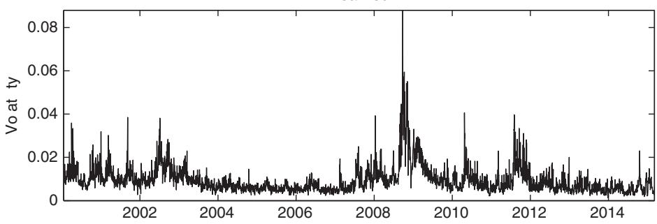
The top window in figure 13.3 provides a plot of daily realized volatilities (the square root of realized variances) on the S&P500 index constructed using fiveminute sampling (obtained from the Oxford-Man institute). There is clear evidence of volatility clustering and outliers such as during the fall of 2008. The bottom window of figure 13.3 shows the predicted volatility from an autoregressive model fitted to the realized volatility series. While these forecasts do not pick up the outliers in the realized series, they are broadly consistent with the movements in the realized series and identify a high level of persistence in this series.

Viewing ${\mathrm{RV}}_t$ as an observed, albeit noisy, estimate of the variance, ${\sigma }_t^2$ , we can go ahead and use many standard forecasting tools to predict future volatility, ${\sigma }_{t+1}^2.$ Typically, RV is found to be highly persistent at daily and longer horizons with autocorrelations that decay only slowly. To capture this property, one option is to model log ${\mathrm{RV}}_t$ as a long-memory process using autoregressive fractionally integrated moving average (ARFIMA) models of the form

AR forecasts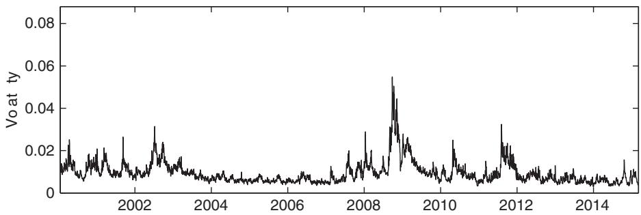

Figure 13.3: Realized volatility versus predicted values from an autoregressive model with lag length selected by the AIC.

$$\varphi (L)(1-L{)}^d\left(\frac{1}{2}\log ({\mathrm{RV}}_t)-\mu \right)={\eta }_t,d\in [0,1],$$

where ${\eta }_t$ is white noise. If $d=0;$ , this amounts to a simple AR model for log(RVt ) with the largest eigenvalue likely to be quite large due to the persistence in the realized variance.

One approach to deal with measurement errors in the volatility measure is to consider the joint dynamics in alternative volatility estimates. Engle and Gallo (2006) develop a multiplicative error forecasting model based on the joint dynamics in daily absolute returns, the daily high–low range and the daily realized volatility.

Another possibility is to add RV terms to GARCH models. For example, the GARCH(1,1) model could be extended to

$${\sigma }_{t+1|t}^2=\omega +{\alpha }_1{\epsilon }_t^2+{\beta }_1{\sigma }_{t|t-1}^2+\gamma {\mathrm{RV}}_t.\text{\hspace{1em}(13.24)}$$

As pointed out by Hansen and Lunde (2011), this can be attractive because the filtration underlying the GARCH estimates is usually based on past returns sampled at a relatively low frequency, whereas the filtration underlying ${\mathrm{RV}}_t$ can be quite different and is based on sampling at a different (higher) frequency.