正在学习
11.2.5 Empirical Illustration
11.2.5 Empirical Illustration
As an illustration of the nonparametric approaches, we consider forecasting the quarterly CPI inflation rate and value-weighted returns on the US stock market using their respective lagged values. We choose these series because they have very different dynamic properties, with inflation having a highly persistent mean, while stock returns have little or no autocorrelation.
Figure 11.1 shows forecasts of inflation and stock returns using kernel bandwidths of b = 0.5σˆ , b = ˆσ , and b = 2σˆ , where σˆ is the estimated standard deviation of the underlying variable. The inflation forecasts are considerably more volatile, the narrower the bandwidth, and the more “local” the weighting under this approach. For , the inflation rate forecasts are quite extreme as they are based on a narrow local average. In contrast, for the range of forecasts falls in a narrower band from 0 to 8% per annum. The sensitivity of the range of predicted value to the choice of bandwidth is equally large for the stock return series for which the volatility of the kernel forecasts is far higher for the smallest bandwidth compared to the largest bandwidth as can be noticed from the difference in scales in the three panels.
Figure 11.2 shows sequences of forecasts generated by artificial neural network models where we use an initial period 1947–1969 to estimate the first set of parameters before recursively expanding the estimation window and generating forecasts out-of-sample over the period 1970–2013. The number of terms in the neural network is selected either by the AIC or by the BIC. The two sets of inflation forecasts are quite similar with a time-series correlation of 0.94.
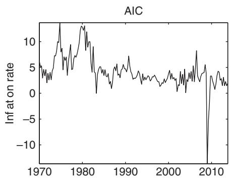
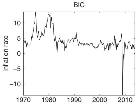
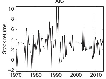
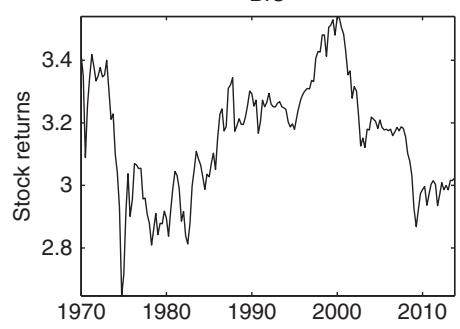
Figure 11.2: Artificial neural network forecasts of inflation and stock returns with network terms selected by the AIC or BIC criteria.
Figure 11.3 shows the number of terms selected by the ANN using either the AIC or the BIC. For the inflation series, the neural network selected by the AIC includes up to 12 terms (the maximum), although it frequently includes far fewer terms. The number of terms selected also tends to vary quite a bit through time. The BIC selects far fewer terms, typically three or four terms. For stock returns, the BIC includes no lags while the AIC typically includes one or two lags.
The top panel in figure 11.4 shows recursively generated inflation rate forecasts from a cubic spline with nodes at the 20th, 40th, 60th, and 80th percentiles. The cubic spline inflation forecasts generate an unexpected negative forecast around 1980 and an extremely large negative value around −0.25 in 2008. Cubic spline forecasts of stock returns, shown in the bottom panel in figure 11.4 also record extreme forecasts, namely a large negative value below −40% in 1970 and a very large positive value above 60% in 1975.
Sensible forecasters would arguably have been skeptical about using such forecasts and might have resorted instead to using a historical average (stock returns) or the previous value (inflation) in place of the extreme forecast. This is akin to using what is sometimes called the “insanity filter” and is a strategy that can be adopted in real time—the forecaster overrules a model-generated forecast if it is too implausible.6
Table 11.1 reports the root mean squared error performance of a range of nonparametric forecasts along with those of a random walk and prevailing mean model. For the inflation rate, the best forecasts are generated by the ANN with terms recursively selected by the BIC. The kernel approaches perform relatively well, although they get worse for the largest value of the bandwidth. The cubic spline results are extremely poor if the outlier forecast is relied on but are otherwise quite good, illustrating the importance of filtering extreme forecasts from such approaches.
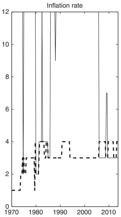
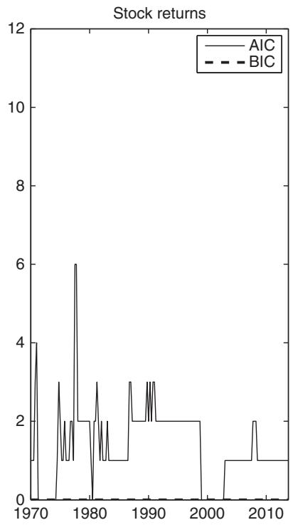
Figure 11.3: Number of terms in the artificial neural network selected by the AIC or BIC models fitted to the inflation rate or stock return forecasts.
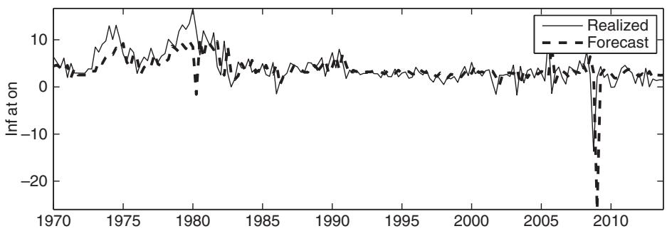
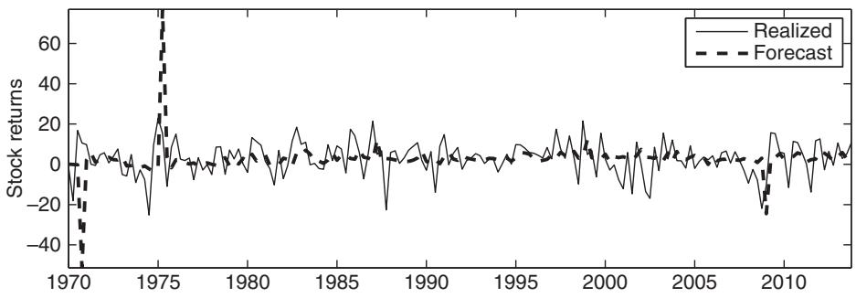
Figure 11.4: Inflation and stock return forecasts using cubic splines.
TABLE 11.1:
Root mean squared error performance for two benchmarks (random walk and prevailing mean) and a range of nonparametric models: artificial neural networks (ANN) with terms selected by the AIC or BIC information criteria, kernel forecasts with three different bandwidths, and cubic spline forecasts using four nodes and truncation of the most extreme forecast (marked Spline**).
| Method | Inflation | Stock |
| Random walk | 3.1646 | 11.4595 |
| Prevailing mean | 3.6395 | 8.4834 |
| ANN(AIC) | 3.0572 | 8.7907 |
| ANN(BIC) | 2.9281 | 8.4878 |
| Kernel | 3.0167 | 10.5425 |
| Kernel | 3.0052 | 9.2402 |
| Kernel | 3.2141 | 8.5243 |
| Spline | 3.6831 | 10.6889 |
| Spline** | 3.0944 | 8.4862 |
For stock returns, the best forecasts are generated by the prevailing mean, closely followed by forecasts from the ANN with terms selected by the BIC and the cubic spline forecasts that truncate extreme values. Turning to the kernel forecasts, the narrower the bandwidth, the worse the forecast, i.e., the nearest neighbors contain very little information on stock returns.
练习题
Which kernel bandwidth results in the narrowest range of inflation forecasts?
What are the characteristics of cubic spline forecasts for stock returns?
The BIC criterion typically selects more terms than the AIC criterion in ANN models for inflation forecasting.
The cubic spline inflation forecasts generate an extremely large negative value around ___ in 2008.
Explain the 'insanity filter' strategy in forecasting.
What is the primary advantage of using projection pursuit regression?
Which statements are true about kernel bandwidths and stock return forecasts?
Artificial neural network forecasts using AIC and BIC criteria for inflation are highly dissimilar with low correlation.
The neural network selected by the AIC for inflation series includes up to ___ terms.
What is the impact of using the largest kernel bandwidth on inflation forecasts?
When using kernel bandwidths for forecasting inflation rates, which bandwidth choice results in the most volatile forecasts and why?
Which of the following statements are true regarding the selection of terms in artificial neural networks (ANNs) for forecasting?
Cubic spline forecasts for stock returns can produce extreme values, such as a large negative value below −40% in 1970 and a very large positive value above 60% in 1975, which supports the use of the 'insanity filter' strategy.
The ___ criterion tends to select fewer terms than the ___ criterion when used in artificial neural networks for forecasting inflation rates.
登录后解锁笔记、知识点解析、AI 问答
立即登录