正在学习
10.5.1 Factor Models versus Bayesian VARs
10.5.1 Factor Models versus Bayesian VARs
In settings with large sets of predictor variables, empirical researchers have traditionally used factor models to generate forecasts. However, as we discussed in chapter 9, studies such as Banbura, Giannone, and Reichlin (2010) develop Bayesian VAR methods that work even with large sets of conditioning variables, e.g., more than 100. Empirically, they find that their Bayesian VARs produce better forecasts than factor-based approaches. Consistent with this, Koop (2013) finds that a common factor approach often produces worse forecasts than Bayesian VARs although the ranking depends on how the trade-off between incorporating more information and dampening the effect of estimation error is implemented across different Bayesian methods.
This highlights important trade-offs between factor models and Bayesian VARs. The performance of the Bayesian VARs can be quite sensitive to the choice of prior and it is clear that the same prior, and thus the degree of shrinkage, does not work well across different economic variables. For some dependent variables, small-scale BVARs work well, corresponding to ignoring the information contained in a large set of predictors. For other dependent variables, it can be important to condition on a larger set of predictors. One important advantage of Bayesian VARs is that they are set up to produce density forecasts as opposed to simple point forecasts. While density forecasts can also be generated from factor models, they require additional assumptions and will typically not account for parameter estimation error in the same way as the Bayesian approach does.
10.5.2 Application
To illustrate the factor approach empirically, we constructed a data set containing 65 variables capturing different aspects of the US economy. The variables include several categories such as industrial production growth, capacity utilization, personal consumption expenditures, retail sales, unemployment and payroll data, housing starts, inventories, inflation, average hourly earnings, commodity and stock price indexes, interest rates, and money supply. In each case we transform the series so it is stationary. The data are monthly and run from 1948:1 to 2010:12.
Figure 10.1 plots time series of the first four principal components extracted from this data set. The first three factors are quite persistent with occasional large shifts in levels, particularly for the second and third factor, while the fourth factor is far less persistent.
We next consider the stability of the factor approach when applied recursively through time. To this end, we report both the proportion of the total variation in the panel of predictor variables that can be explained by the first four factors, the number of factors selected by the forecasting models, along with the forecasts based on the factor models, and their resulting out-of-sample performance.
Figure 10.2 plots the fraction of the explained variance over time. The first factor accounts for close to 50% of the variance, while factor two accounts for between 20 and 25%. The third factor accounts for between 15 and 20% of the variation, while the fourth factor accounts for close to 12%. Thus, while the proportion of the variance explained by the first and fourth factors is quite stable through time, it is less stable for the second and third factors, although the total variation explained jointly by these two factors is fairly constant through time, adding up to a little less than 40%.
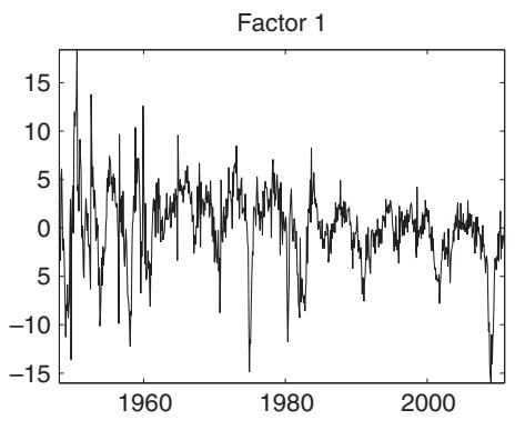
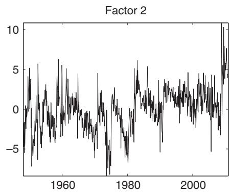
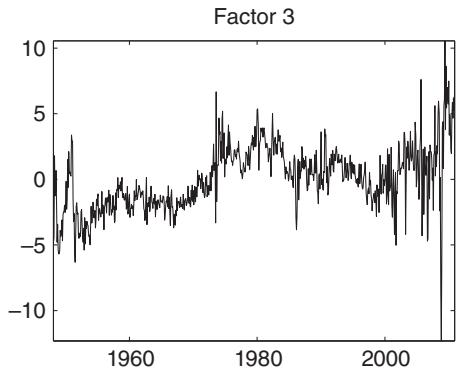
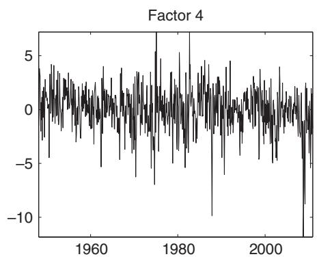
Figure 10.1: First four common factors extracted from a sample of macroeconomic and financial variables.
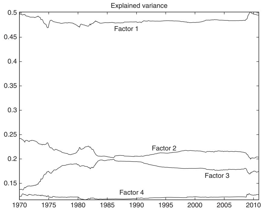
Figure 10.2: Recursive estimates of the proportion of the common variation explained by the first four factors.
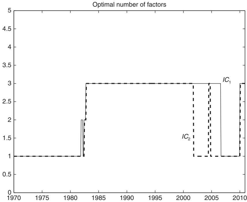
Figure 10.3: Number of factors chosen by the Bai and Ng selection criteria applied recursively through time.
For the pure factor models, figure 10.3 shows that the two information criteria and select a fairly modest number of common factors which varies between one and three.
Figures 10.4 and 10.5 show monthly forecasts for the inflation rate and unemployment rate series. We use the sample 1948:01–1969:12 for initial parameter estimation and the period 1970:01–2010:12 to evaluate the forecasts out-of-sample.
We show results for pure factor models including either models that include one or four factors, a VAR, a dynamic factor model, and two Ridge regressions with small and large penalty terms, respectively. For each variable, the single factor forecast is generally quite smooth, particularly when compared against the forecast with multiple factors. The VAR and dynamic factor model (DFM) forecasts are nearly identical, suggesting that once autoregressive terms are included, the factor terms are relatively less important. Among the Ridge forecasts, the effect of applying a heavy penalty term is to substantially smooth the forecasts.
Table 10.1 reports the forecasting performance of factor models selected by or in addition to principal components models with one or four factors, Ridge regressions, a VAR(1), a VAR with lag length selected by the AIC, dynamic factor models, and random walk and prevailing mean benchmarks.
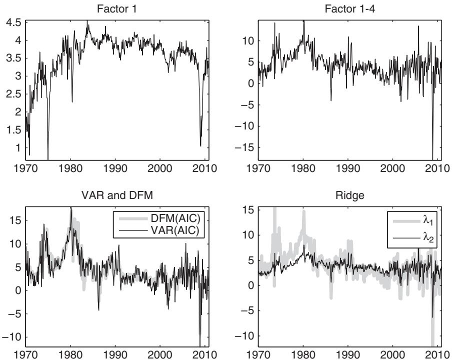
Figure 10.4: Recursive forecasts of the inflation rate using different combinations of the factors (top), a VAR and a factor-augmented VAR, and Ridge regression (bottom).
For the inflation rate series, the best models are the univariate autoregressive models closely followed by the VAR and DFM specifications, all of which beat the random walk benchmark. The pure factor models do comparatively worse with RMSE values above those of the best models, although the model that includes four factors still beats the random walk benchmark. This highlights the importance of including autoregressive terms for many macroeconomic variables. The performance of the Ridge regressions depends on the value of the penalty or shrinkage factor with weak amounts of shrinkage working best for this series. For stock returns, the Ridge regression with the largest amount of shrinkage is the only method that performs better than the benchmark prevailing mean method, although a number of approaches register RMSE performance similar to this benchmark. For stock returns, the most parsimonious models generate the most accurate forecasts, consistent with earlier findings for this variable.
The best unemployment rate forecasts come from the dynamic factor models, followed closely by the AR and VAR forecasts. Pure factor-based forecasts perform poorly again as they fail to pick up the very high persistence in this series. A similar conclusion holds for the T-bill rate, for which the AR, VAR, and dynamic factor models perform best, while the pure factor and Ridge models produce poor out-ofsample forecasts.
Table 10.2 reports Diebold–Mariano test statistics comparing the mean squared error performance of the forecasts in the previous table against a benchmark model. For persistent variables such as the inflation rate, unemployment, and the T-bill rate, the random walk model is a reasonable benchmark. Conversely, for
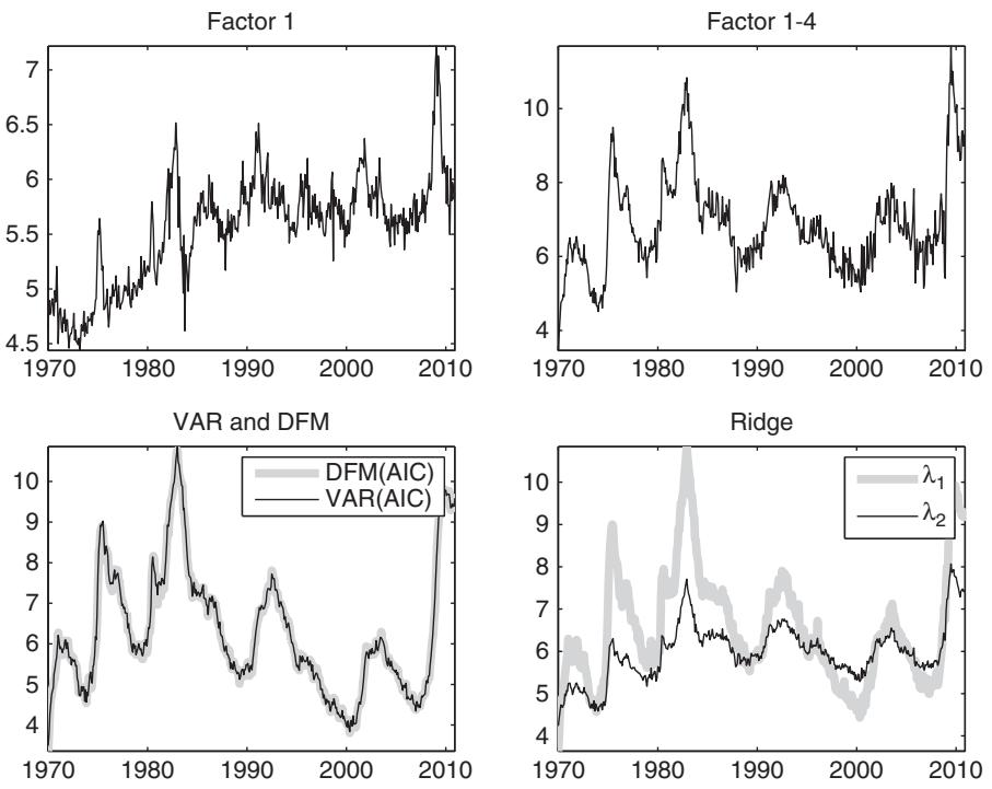
Figure 10.5: Recursive forecasts of the unemployment rate using different combinations of the factors (top), a VAR, a dynamic factor model, and Ridge regression (bottom).
TABLE 10.1:
Out-of-sample root mean squared forecast error performance for different models used to predict the monthly inflation rate, stock returns, unemployment rate, and the short interest rate. AR refers to univariate autoregressive models with lag length selected by the AIC or BIC, Ridge refers to Ridge regression, PC refers to principal components methods with the number of factors selected by the information criteria of Bai and (2002) and , one principal component , four principal components , vector autoregressions (VAR(AIC) and VAR(1)), and two dynamic factor models (DFM(AIC), DFM(1)).
| Method | Inflation | Stock | Unemployment | Interestrate |
| Random walk | 3.4581 | 6.2488 | 0.1835 | 0.5001 |
| Prevailing mean | 4.2462 | 4.5388 | 1.8031 | 3.4816 |
| AR(AIC) | 3.0279 | 4.5720 | 0.1744 | 0.4978 |
| AR(BIC) | 3.1065 | 4.5390 | 0.1727 | 0.4901 |
| Ridge, | 3.1069 | 4.5917 | 0.4721 | 2.1419 |
| Ridge, | 3.5641 | 4.5269 | 1.1647 | 3.0255 |
| PC (IC1) | 4.3079 | 4.5380 | 1.4095 | 3.5074 |
| 4.2546 | 4.5406 | 1.3675 | 3.4308 | |
| 4.2062 | 4.5393 | 1.6985 | 3.4707 | |
| 3.3065 | 4.5592 | 0.9504 | 2.9615 | |
| 3.1260 | 4.6694 | 0.1769 | 0.4869 | |
| 3.0743 | 4.5742 | 0.1856 | 0.5061 | |
| 3.2278 | 4.7372 | 0.1626 | 0.4763 | |
| DFM(1) | 3.1252 | 4.6033 | 0.1575 | 0.4845 |
TABLE 10.2:
Diebold–Mariano test statistics for quarterly out-of-sample mean squared error performance measured relative to the random walk benchmark for the inflation, unemployment, and interest rate series and relative to the prevailing mean benchmark for stock returns.
| Method | Inflation | Stock | Unemployment | Interestrate |
| Random walk | 0.0000 | -7.0860 | 0.0000 | 0.0000 |
| Prevailing mean | -2.6991 | 0.0000 | -7.8383 | -7.5985 |
| AR(AIC) | 2.4778 | -1.0894 | 1.9847 | 0.0793 |
| AR(BIC) | 2.1590 | -1.6005 | 2.3919 | 0.4114 |
| 3.5015 | -0.7848 | -10.4994 | -8.1223 | |
| -0.5370 | 0.7163 | -9.2411 | -8.1120 | |
| -3.1299 | 0.0347 | -9.6665 | -7.8576 | |
| PC (IC2) | -2.8699 | -0.0922 | -8.3682 | -7.4224 |
| -2.6468 | -0.0322 | -8.3236 | -7.5509 | |
| 1.5718 | -0.6082 | -11.0552 | -9.1946 | |
| VAR(AIC) | 2.0430 | -2.0898 | 0.9606 | 0.5711 |
| VAR(1) | 2.6658 | -0.8326 | -1.0256 | -1.4500 |
| DFM(AIC) | 1.8846 | -2.9401 | 2.5033 | 1.0641 |
| DFM(1) | 3.1808 | -1.4957 | 3.3383 | 2.0652 |
stock returns that are not serially correlated, a better benchmark is the prevailing mean. Once again, for the stock return series there is no evidence that any of the forecasting methods is capable of beating the prevailing mean forecast’s mean squared error performance. In contrast, the dynamic factor models in particular generate substantially more accurate point forecasts than the random walk forecasts for the inflation, unemployment, and interest rate series. For the inflation and unemployment rate series there is also evidence that the univariate AR models beat the benchmark random walk.
These results indicate that, for the data considered here, once autoregressive terms have been included in the forecasting model, there is little evidence that adding factors improves on the accuracy of the forecasts.
练习题
Which of the following statements is true regarding the performance of Bayesian VARs and factor models in large predictor sets?
What is one key advantage of Bayesian VARs over factor models in forecasting?
Which of the following are true about the trade-offs in Bayesian VARs performance? (Select all that apply)
Bayesian VARs are less sensitive to the choice of prior compared to factor models.
Density forecasts generated from factor models typically account for parameter estimation error in the same way as Bayesian VARs.
The performance of Bayesian VARs can be quite sensitive to the choice of ___.
One advantage of Bayesian VARs is their ability to produce ___ forecasts.
Explain why the performance of Bayesian VARs can vary across different economic variables.
How do Bayesian VARs account for parameter estimation error in density forecasts compared to factor models?
What is the approximate percentage of variance explained by the first factor in the data set constructed for the factor approach?
Which of the following statements are true about the persistence of principal components? (Select all that apply)
The proportion of variance explained by the second factor is more stable over time than that explained by the first factor.
The first factor accounts for close to ___% of the variance in the data set.
The fourth factor accounts for close to ___% of the variance.
Explain the stability of the variance explained by the first and fourth factors over time compared to the second and third factors.
Describe the persistence of the first four principal components extracted from the data set.
Which of the following is NOT a category of variables included in the data set constructed for the factor approach?
Which of the following are true about the data set constructed for the factor approach? (Select all that apply)
The data set constructed for the factor approach includes variables measured at different frequencies.
The data set constructed for the factor approach contains ___ variables.
What is the purpose of transforming the series in the data set to be stationary?
Which of the following statements is true regarding the number of factors selected by the Bai and Ng criteria?
Which of the following are true about the forecasts for inflation and unemployment rates? (Select all that apply)
The single factor forecast for inflation and unemployment rates is generally quite smooth compared to forecasts with multiple factors.
The VAR and dynamic factor model (DFM) forecasts for inflation and unemployment rates are nearly ___.
Explain the effect of applying a heavy penalty term in Ridge regressions on the forecasts for inflation and unemployment rates.
What is the significance of the Bai and Ng criteria in selecting factors for forecasting?
Which of the following is a key consideration when choosing between static and dynamic factor models?
Which of the following statements are true about generalized shrinkage methods compared to dynamic factor models? (Select all that apply)
When comparing Bayesian VARs and factor models for forecasting macroeconomic variables, which of the following statements is most accurate based on empirical findings?
Which of the following statements correctly describe advantages of Bayesian VARs over factor models in forecasting applications? (Select all that apply)
The empirical success of factor models in forecasting is uniform across all types of economic variables, with particularly strong performance for nominal variables like inflation rates.
Explain why Bayesian VARs might be preferred over factor models when forecasting a small set of economic variables with well-established theoretical relationships, even though factor models generally perform better with large predictor sets.
登录后解锁笔记、知识点解析、AI 问答
立即登录