9.3.7 Empirical Example: Asset Allocation with Return Predictability

9.3.7 Empirical Example: Asset Allocation with Return Predictability

To illustrate the use of Bayesian VAR methods, we next return to the empirical asset allocation example from section 3.5 but in a setting that, following Barberis (2000), allows for return predictability and so introduces a market timing component in the investor’s decision process. Specifically, suppose that the continuously compounded stock returns, ${\mathbf{r}}_t,$ measured in excess of a risk-free asset paying $r_f,$ , contain a predictable component which is captured through a single predictor variable, $x_t.$ , and assume that $y_t^{\prime }=(r_t,x_t)$ follows a first-order VAR:

$$y_t=c+A_1{y}_{t-1}+{\epsilon }_t,{\epsilon }_t\sim \mathrm{ind}N(0,\Sigma ).\text{\hspace{1em}(9.31)}$$

Under the classical approach the VAR parameters $\theta =(c,A_1,\Sigma )$ can be estimated and the VAR in (9.31) can be iterated forward conditional on these parameter estimates. This generates a distribution of future cumulative stock returns conditional on the parameter values, $\begin{array}{r}{p}_Y({\sum }_{\tau =1}^h{y}_{\tau }|Z_T,\hat{\theta })\end{array}$ , where $Z_T=(y_1,\dots ,y_T)$ is the observed data vector. Specifically,

$$\begin{array}{l}{y}_{T+h}=c+A_{1}c+A_1^{2}c+\cdot \cdot \cdot +A_1^{h-1}c\\ +A_1^h{y}_T+{\epsilon }_{T+h}+A_1{\epsilon }_{T+h-1}+A_1^2{\epsilon }_{T+h-2}+\cdot \cdot \cdot +A_1^{h-1}{\epsilon }_{T+1}.\end{array}\text{\hspace{1em}(9.32)}$$

Conditional on $c,A_1,\Sigma$ , from (9.32) the sum $y_{T+1:T+h}\equiv y_{T+1}+y_{T+2}+\cdot \cdot \cdot +y_{T+h}$ is normally distributed with mean and variance (see Barberis (2000))

$$\begin{array}{rl}& \begin{array}{rl}& E[y_{T+1:T+h}|\theta ]=hc+(h-1)A_{1}c+(h-2)A_1^{2}c+\cdot \cdot \cdot +A_1^{h-1}c\\ & +(A_1+A_1^2+\cdot \cdot \cdot +A_1^h)z_T,\end{array}\\ & \begin{array}{rl}& +(A_1+A_1^2+\cdot \cdot \cdot +A_1^h)z_T,\\ & \\ & \mathrm{Var}[y_{T+1:T+h}|\theta ]=\Sigma \end{array}\\ & \begin{array}{rl}& +(I+A_1)\Sigma (I+A_1{)}^{\prime }\\ & +(I+A_1+A_1^2)\Sigma (I+A_1+A_1^2{)}^{\prime }\\ & ⋮\\ & ⋮\\ & +(I+A_1+A_1^2+\cdot \cdot \cdot +A_1^{h-1})\Sigma (I+A_1+A_1^2+A_1^{h-1}{)}^{\prime }.\end{array}\end{array}\text{\hspace{1em}(.33)}$$

Using these expressions and plugging in parameter estimates $\hat{\theta }=(\hat{c},{\hat{A}}_1,\hat{\Sigma })$ , the classical investor maximizes the expected utility of future wealth $u(W_{T+h})$ , where

$$\underset{\omega \in [0,1)}{\max }\int d\cdot \cdot \cdot \int u(W_{T+h}{)}_{\hat{P}Y}(\sum _{\tau =1}^h{y}_{T+\tau }|Z_T,\hat{\theta })d{y}_{1,T+1}\dots d{y}_{1,T+h},\text{\hspace{1em}(9.34)}$$

where $y_{1,T+\tau }=e_1^{\prime }{y}_{T+\tau }$ selects the first element of ${\gamma }_{T+\tau }$ and where future wealth is given by

$$W_{T+h}=(1-\omega (z))\exp (r_{f}h)+\omega (z)\exp \left(r_{f}h+\sum _{\tau =1}^h{y}_{T+\tau }\right).\text{\hspace{1em}(9.35)}$$

The Bayesian approach conditions only on the data and so uses the following posterior density to compute expected utility:

$$p_Y\left(\sum _{\tau =1}^h{y}_{1,T+\tau }|Z_T\right)=\int p_Y\left(\sum _{\tau =1}^h{y}_{T+\tau }|Z_T,\theta \right)p(\theta |Z_T)d\theta .\text{\hspace{1em}(9.36)}$$

To draw from the posterior return distribution, $\begin{array}{r}p(c,A_1,\Sigma |Z_T)\end{array}$ , write the model as

$$\left(\genfrac{}{}{0ex}{}{y_2^{\prime }}{⋮}\right)=\left(\begin{array}{cc}1& y_1^{\prime }\\ ⋮& ⋮\\ y_T^{\prime }& \end{array}\right)\left(\begin{array}{c}{c}^{\prime }\\ A_1^{\prime }\end{array}\right)+\left(\begin{array}{c}{\epsilon }_2^{\prime }\\ ⋮\\ {\epsilon }_T^{\prime }\end{array}\right),$$

or, in more compact form,

$$\begin{array}{r}Y=Z\beta +U,\end{array}$$

where Y is a $((T-1)\times 2)$ matrix with the vectors $y_2^{\prime },\dots ,y_T^{\prime }$ as rows. Assuming a single predictor variable, Z is a $((T-1)\times 2)$ matrix with the vectors $(1,y_1^{\prime }),\dots ,(1,y_{T-1}^{\prime })$ as rows; and U is a $((T-1)\times (n+1))$ matrix with the vectors ${\epsilon }_2^{\prime },\dots ,{\epsilon }_T^{\prime }$ as rows. The matrix $\beta$ is $(2\times 2)$ with top row $c^{\prime }$ and the matrix $A_1^{\prime }$ below that.

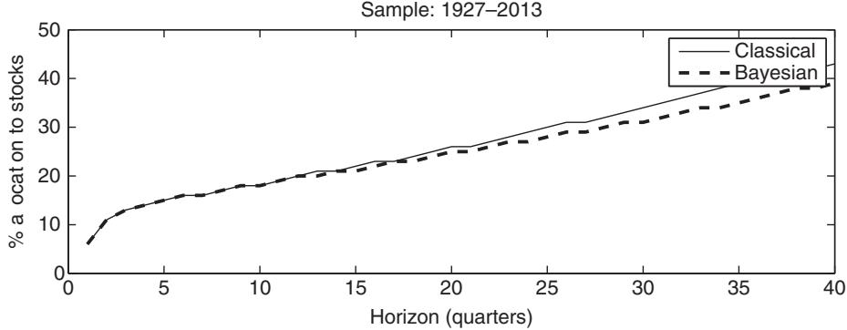
Figure 9.1: Percentage allocation to stocks for different holding periods in the presence of return predictability from the dividend yield.

To sample from the Bayesian predictive distribution, we first generate a sample of size I from the posterior distribution for the parameters, $\begin{array}{r}p(c,A_1,\Sigma |Z_T)\end{array}$ . For each set of parameter values drawn, ${\theta }^i=\{c^i,A_1^i,\overline{{\Sigma }^i}\}$ , we sample from the distribution of returns conditional on $Z$ and ${\theta }^i$ . Assuming uninformative priors, Barberis (2000) shows that the posterior of the parameters are given by

$$p({\Sigma }^{-1}|Z_T)\sim \mathrm{Wishart}(T-n-2,S^{-1}),$$

$$p(\mathrm{vec}(\beta )|\Sigma ,Z_T)\sim N(\mathrm{vec}(\hat{\beta }),\Sigma \otimes (Z^{\prime }Z{)}^{-1}),$$

where $S=(Y-Z\hat{\beta }{)}^{\prime }(Y-Z\hat{\beta })$ with $\hat{\beta }=(Z^{\prime }Z{)}^{-1}{Z}^{\prime }Y$ . Samples from the posterior return distribution are generated by first drawing from the marginal distribution, $p({\Sigma }^{-1}|Z_T)$ , then drawing from the conditional distribution $p(C|\Sigma ,Z_T)$ . For each draw of parameters from the posterior $\begin{array}{r}p(c,A_1,\Sigma |Z_T)\end{array}$ , we generate a single draw from the normal distribution with mean and variance given by (9.33). Repeating this many times gives a large sample from the predictive return distribution.

Empirical results for the case with return predictability from the dividend yield— the predictor variable used by Barberis (2000)—are presented in figure 9.1. To show the importance of the length of the estimation sample, the top figure uses quarterly returns data over the sample 1927–2013, while the bottom window uses a shorter 20-year data sample from 1994–2013. The results assume a coefficient of relative risk aversion of 5 and power utility, i.e., the objective function in equation (3.33). We set the risk-free rate and the dividend yield at their values as of the end of the sample.

First consider the long estimation sample (top). Since a lot of data are available to estimate model parameters, we observe only small differences in the allocations under the classical and Bayesian approaches. In both cases the allocation to stocks increases as the forecast horizon grows longer. In contrast, the two allocations are very different under the classical and Bayesian approaches when the 20-year estimation sample is used (bottom). In this case, long-run investors will allocate a considerably smaller amount to stocks under the Bayesian approach (which accounts for parameter estimation uncertainty) than under the classical approach (which ignores such uncertainty).

The nonmonotonic pattern seen in the shorter sample (1994–2013) reflects two distinct effects. First, the value of the dividend yield that the model conditions on at the point of the investment decision is quite low relative to the sample mean of the predictor. Given the positive relation between the dividend yield and predicted stock returns, this reduces expected returns, particularly at short to medium horizons. On the other hand, the dividend yield captures a slowly, mean-reverting component in stock returns which makes stock returns less risky particularly at the longer horizons where this effect dominates.

A very different pattern is observed for the Bayesian investor whose allocation to stocks falls uniformly from close to 70% at the one-month horizon to less than 40% at the longest five-year horizon. For this investor, the effect of estimation error clearly does not get reduced as the investment horizon gets extended.