8.3.1 Forecasting with Regime Switching Models

8.3.1 Forecasting with Regime Switching Models

Forecasting the first-order Markov chain is straightforward. Following Hamilton (1994) let the $(K\times 1)$ vector ${\xi }_t$ be a random indicator variable that tracks the current regime, i.e.,

$$\begin{array}{cc}{\xi }_t=(1,0,0,\dots ,0{)}^{\prime }& \mathrm{if}{s}_t=1,\\ {\xi }_t=(0,1,0,\dots ,0{)}^{\prime }& \mathrm{if}{s}_t=2,\\ ⋮& ⋮\\ {\xi }_t=(0,0,\dots ,0,1{)}^{\prime }& \mathrm{if}{s}_t=K.\end{array}$$

Under the assumption of constant transition probabilities in (8.16), ${\xi }_{t+1}$ can be written as a VAR(1) in state space form:

$${\xi }_{t+1}=P{\xi }_t+v_{t+1},\text{\hspace{1em}(8.17)}$$

where ${\mathbf{v}}_{t+1}={\xi }_{t+1}-E\left[{\xi }_{t+1}|{\xi }_t,{\xi }_{t-1},...\right]$ is a martingale difference sequence, i.e.,

$$E\left[v_{t+1}|v_t,v_{t-1},...\right]=0.$$

Iterating on (8.17), we have

$$\begin{array}{rl}& {\xi }_{t+h}=P{\xi }_{t+h-1}+v_{t+h}\\ & =P(P{\xi }_{t+h-2}+v_{t+h-1})+v_{t+h}\\ & =(P\times P){\xi }_{t+h-2}+P{v}_{t+h-1}+v_{t+h}\\ & =P^h{\xi }_t+v_{t+h}+P{v}_{t+h-1}+\cdot \cdot \cdot +P^{h-1}{v}_{t+1},\end{array}$$

$$\begin{array}{rl}{s}_0& E\left[{\xi }_{t+h}|{\xi }_t\right]=P^h{\xi }_t.\end{array}\text{\hspace{1em}(8.18)}$$

Here $P^h={\prod }_{t=1}^{h}P$ is P multiplied by itself h times. The h-period-ahead transition probabilities are thus obtained by multiplying P by itself h times and the probability that an observation from regime i is followed h periods later by an observation from regime j , $P(S_{t+h}=j|S_t=i)$ is given by the row i , column j element of the matrix ${\check{P}}^h$

For the two-state model $\left(K=2\right)$ , forecasts of future regime probabilities take the simple form (see Hamilton, 1994)

$$\begin{array}{r}{P}^h=\left[\begin{array}{cc}\frac{(1-p_{22})+(p_{11}+p_{22}-1{)}^h(1-p_{11})}{2-p_{11}-p_{22}}& \frac{(1-p_{22})-(p_{11}+p_{22}-1{)}^h(1-p_{22})}{2-p_{11}-p_{22}}\\ \frac{(1-p_{11})-(p_{11}+p_{22}-1{)}^h(1-p_{11})}{2-p_{11}-p_{22}}& \frac{(1-p_{11})+(p_{11}+p_{22}-1{)}^h(1-p_{22})}{2-p_{11}-p_{22}}\end{array}\right].\end{array}\text{\hspace{1em}(8.19)}$$

From this we can see that the key to the long-term regime forecasts is the “overall” persistence measure $(p_{11}+p_{22}-1)$ . The two-state process is in fact positively autocorrelated if $p_{11}+p_{22}>1$ and the bigger is $p_{11}+p_{22}-1$ , the more persistent the process.

In practice, the underlying states are unobserved and so regime switching forecasts rely on estimated state probabilities. Once again, the forecast becomes a weighted average of forecasts conditional on the respective regimes with weights reflecting the predicted state probabilities. In the case with two states, we have from (8.15),

$$\begin{array}{rl}& f_{t+1|t}(z)={\mu }_1\left[{\hat{p}}_{1t}{p}_{11}+(1-{\hat{p}}_{1t})(1-{\hat{p}}_{22})\right]\\ & \\ & +{\mu }_2\left[{\hat{p}}_{1t}(1-{\hat{p}}_{11})+(1-{\hat{p}}_{1t})p_{22}\right],\end{array}\text{\hspace{1em}(8.20)}$$

where ${\hat{p}}_{1t}$ is the estimated probability of being in regime 1 at time t using data up to time t and so itself depends on the entire data set up to time t.

Recursive updates to the state probabilities will affect the forecasts even if the parameters are known, as the next example shows.

Example 8.3.1 (Recursive updates of state probabilities). If the model parameters $\theta =({\mu }_1,{\mu }_2,{\sigma }^2,p_1,p_2{)}^{\prime }$ are known and ${\epsilon }_t\sim ind\mathrm{N}(0,{\sigma }^2)$ , the state probabilities can be derived recursively as shown by Hamilton (1994, page 692). Let $p_{t|t}\equiv \left(p_{1t|t}\frac{p_{2t|t}}{p_{2t|t}|}\right)=$ $(\mathrm{Pr}(S_t=1|y_t,y_{t-1},\dots ),\mathrm{Pr}(S_t=2|y_t,y_{t-1},\dots ){)}^{\prime }$ , while $p_{t+1|t}\equiv ({\mathbf{p}}_{1t+1|t}{\mathbf{p}}_{2t+1|t})=$ $(\mathrm{Pr}(S_{t+1}=1|y_t,y_{t-1},\dots ),\mathrm{Pr}(S_{t+1}=2|y_t,y_{t-1},\dots ){)}^{\prime }$ be the conditional probabilities for the current and future state given the observed history of realizations. These evolve

according to the equations

$$\begin{array}{rl}& {\dot{p}}_{t\mid t}=\frac{{\dot{p}}_{t\mid t-1}\odot \left(\begin{array}{l}\exp (-\frac{(y_t-{\mu }_1{)}^2}{2{\sigma }^2})/\sqrt{2\pi {\sigma }^2}\\ \exp (-\frac{(y_t-{\mu }_2{)}^2}{2{\sigma }^2})/\sqrt{2\pi {\sigma }^2}\end{array}\right)}{{\dot{p}}_{1t\mid t-1}\exp (-\frac{(y_t-{\mu }_1{)}^2}{2{\sigma }^2})/\sqrt{2\pi {\sigma }^2}+{\dot{p}}_{2t\mid t-1}\exp (-\frac{(y_t-{\mu }_2{)}^2}{2{\sigma }^2})/\sqrt{2\pi {\sigma }^2}},\\ & {\dot{p}}_{t+1\mid t}=\left(\begin{array}{ll}{\dot{p}}_1& 1-{\dot{p}}_2\\ 1-{\dot{p}}_1& {\dot{p}}_2\end{array}\right){\dot{p}}_{t\mid t}.\end{array}\text{\hspace{1em}(8.21)}$$

where is the Hadamard product. The recursions can be started using initial values such as $p_{0|0}=\pi$

Estimation of regime switching models is typically based on either maximum likelihood or Bayesian methods and assumes that the likelihood is Gaussian within each regime. The likelihood itself is quite complicated but can be written in statespace form and hence a recursive algorithm similar to the Kalman filter can be used to construct the sequences of probability forecasts and forecasts of ${\gamma }_t$ as well.

Example 8.3.2 (Multistep forecasts for the two-state Markov switching process). For many Markov switching models, multistep forecasts can be derived in closed form, at least when parameter estimation uncertainty is ignored. For example, Clements and Krolzig (1998) analyze the following two-state model with first-order autoregressive dynamics:

$$\Delta y_{t+1}-{\mu }_{s_{t+1}}=\alpha (\Delta y_t-{\mu }_{s_t})+u_{t+1},u_{t+1}\sim ind\mathrm{N}(0,{\sigma }_u^2).\text{\hspace{1em}(8.23)}$$

Define the variable ${\zeta }_t=1-\mathrm{Pr}(s_t=2),if{s}_t=2$ otherwise ${\zeta }_t=-\mathrm{Pr}(s_t=2)$ which tracks the state of the hidden Markov chain. The forecast of ${\zeta }_{t+h}$ given information at time t takes the form

$${\hat{\zeta }}_{t+h|t}=(p_{11}+p_{22}-1{)}^h{\hat{\zeta }}_{t|t}.$$

Clements and Krolzig use this to show that the forecast of $\Delta y_{t+h}$ above its unconditional mean, ${\mu }_{y:}$ , is given by

$$\Delta y_{t+h}-{\mu }_y={\alpha }^h(\Delta y_t-{\mu }_y)+({\mu }_2-{\mu }_1)[(p_{11}+p_{22}-1{)}^h-{\alpha }^h]{\hat{\zeta }}_{t|t}.\text{\hspace{1em}(8.24)}$$

The expression in (8.24) is helpful for understanding when forecasts from a Markov switching process such as that in (8.23) can be expected to improve upon forecasts from a simple AR model and when they cannot. First notice that the first term in (8.24) is identical to that from a regular AR(1) model. Only the second term differentiates the Markov switching forecast from the regular AR(1) prediction. This second term will tend to be small if $|{\mu }_2-{\mu }_1|$ is small, i.e., if the means in the two states are similar, or if the persistence of the underlying states as measured by $p_{11}+p_{22}-1$ is not very different from α. 1 A third reason for the two forecasts to be similar arises if the states are not well identified so that ${\hat{\zeta }}_{t\mid t}$ is mostly constant over time. In this case, the second term in (8.24) can be picked up through a constant. Conversely, for the Markov switching process to produce better forecasts, ${\mu }_2$ and ${\mu }_1$ should be quite different, the persistence of the regime switching process should differ from α and the conditional state probabilities should be well identified by the filter.

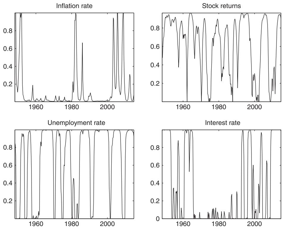
Figure 8.3: Smoothed-state probabilities for two-state Markov switching models.