6.8 PROPERTIES OF MODEL SELECTION PROCEDURES

6.8 PROPERTIES OF MODEL SELECTION PROCEDURES

Choosing a model selection procedure requires a detailed understanding of how such methods work and the extent to which they possess desirable properties. Different notions of what a “good” selection procedure might achieve exist and, as we shall see, these are not always mutually consistent.

If the true model $M^{\ast }=f^{\ast }(z_t,\beta )$ mirroring the data-generating process is included in the set of prediction models under consideration, ${\mathcal{M}}_K=\{M_k=f_k(z_t,{\beta }_k)$ $k=1,\dots ,K\}$ , the notion of consistent model selection becomes meaningful. $\mathrm{A}s-$ suming a discrete set of models, consistent model selection means that $P[\hat{M}=$ $M^{\ast }]1$ as the sample size gets large, where $\hat{M}$ is the selected model. Methods in common use typically have one of two outcomes by this criterion—either they are consistent model selectors or, alternatively, they imply a positive probability of picking too large a model and so are conservative. Selection techniques with a positive asymptotic probability of underfitting the model are rarer.

Cumulated portfolio value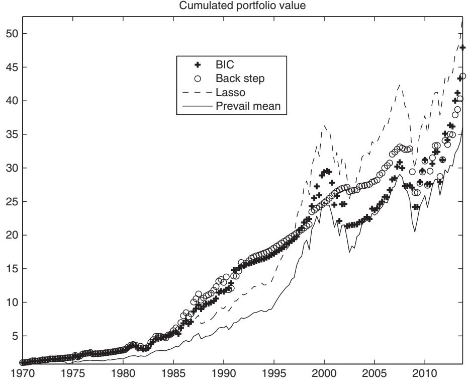

Figure 6.6: Cumulated wealth associated with different forecasting models.

Standard methods for proving consistency of model selection partition the set of models into three sets, ${\mathcal{M}}_K=\{M^{\ast },{\mathcal{M}}_K^{\mathfrak{u}},{\mathcal{M}}_K^{\mathfrak{o}}\}$ , where ${\mathcal{M}}_K^{\mathrm{u}}$ is the set of models that underfit (exclude variables present in the data-generating process, $M^{\ast })$ , and ${\mathcal{M}}_K^0$ is the set of models that overfit (include extraneous variables in addition to those appearing in the true model, $M^{\ast })$ . The proof then shows that $P[\hat{M}\in {\mathcal{M}}_K^{\mathrm{u}}]\to 0$ and $P[\hat{M}\in {\mathcal{M}}_K^{\mathrm{o}}]0$ as the sample size gets large.

Sequential hypothesis testing is typically not a consistent model selection method and tends to overstate the size of the forecasting model. This can best be demonstrated by considering the choice between two linear regression models, one with $n_{k_1}$ regressors and the other with $n_{k_2}>n_{k_1}$ regressors. The smaller model gets selected if we reject a hypothesis test (e.g., a likelihood ratio test) for the null that the additional coefficients in the larger model are 0. Suppose the larger model is the true model. Then the probability of rejecting the null hypothesis—which equals the probability of selecting the larger (true) model—equals the power of the test. For any consistent test, power goes to 1 asymptotically, and so the probability of underfitting goes to 0. Conversely, if the smaller model is the true model, the probability of rejecting the null hypothesis and hence choosing the smaller (true) model is equal to the size of the test. Standard hypothesis tests control the size to remain nonzero asymptotically, so the probability of overfitting $(i.e.,$ choosing the larger model when the smaller one is the true model) is asymptotically equal to the size of the test which is nonzero. Hence, there is a positive probability of overfitting the model, even asymptotically. Computing the extent to which this overfit happens is difficult and method-dependent for more complicated model selection processes, but the basic insight continues to hold.

To gain a heuristic understanding of the types of results that arise for information criteria, we establish model consistency for the general multivariate linear prediction model with n variables:

$$y_{t+1}=A{x}_t+{\epsilon }_{t+1}.\text{\hspace{1em}(6.36)}$$

Here, $y_{t+1}$ is an $n\times 1$ vector and $x_t$ is an $n\times n_k$ matrix. This setup is not as general as that used in the construction of the information criteria. But, it is general enough to cover the majority of uses of information criteria encountered in practical forecasting situations. Specifically, it covers vector autoregressions (VARs), where $x_t$ captures lagged values of $y,$ in addition to general linear systems of equations which are obtained by inserting 0s into the A matrix. Let $n_k$ denote the total number of variables in the model, e.g., in a VAR there are $\mathbf{p}$ lags of n variables and so $n_k=n^{2}p$ when all lags are included, $n_k=n^2(p-1)$ when the pth lag is excluded, and so on. Finally, let ${\hat{\Sigma }}_k$ denote the covariance matrix of the model’s sum of squared residuals.

As we saw in (6.11), ICs choose the model (indexed by $k)$ to minimize $\mathrm{IC}(k)=$ ln $|{\hat{\Sigma }}_k|+h(n_k)g(T)$ . ICs differ over their choice of $g(T)$ and this term plays a crucial role in determining whether a particular information criterion leads to consistent model choice. To establish when an IC is consistent, note from (6.11),

$$\begin{array}{rlr}& & \mathrm{IC}(k)-\mathrm{IC}(k_0)=\ln |{\hat{\Sigma }}_k|+h(n_k)g(T)-\ln |{\hat{\Sigma }}_{k_0}|-h(n_{k_0})g(T)\\ & & =\left(\ln |{\hat{\Sigma }}_k|-\ln |{\hat{\Sigma }}_{k_0}|\right)+\left(h(n_k)-h(n_{k_0})\right)g(T).\end{array}\text{\hspace{1em}(6.37)}$$

Consider first the case with an overfitted model, $n_k>n_{k_0}$ , where $n_{k_0}$ is the number of parameters of the true model. In this case the additional model parameters— over and above the $n_{k_0}$ parameters—are 0 in population. Under normality, −2T $\left\{\ln |{\hat{\Sigma }}_k|-\ln |{\hat{\Sigma }}_{k_0}|\right\}$ is the usual likelihood ratio test statistic for testing that these coefficients are 0. Under standard conditions this converges to an $O_P(1)$ random variable, and hence we have

$$\begin{array}{rl}& P\left(\left(\ln |{\hat{\Sigma }}_k|-\ln |{\hat{\Sigma }}_{k_0}|\right)+(h(n_k)-h(n_{k_0}))g(T)>0\right)\\ & =P\left(\left(\ln |{\hat{\Sigma }}_k|-\ln |{\hat{\Sigma }}_{k_0}|\right)>(h(n_{k_0})-h(n_k))g(T)\right)\\ & =P\left(-2T\left(\ln |{\hat{\Sigma }}_k|-\ln |{\hat{\Sigma }}_{k_0}|\right)<2(h(n_k)-h(n_{k_0}))Tg(T)\right).\end{array}\text{\hspace{1em}(6.38)}$$

For this to converge to 1, we require that $2(h(n_k)-h(n_{k_0}))Tg(T)\infty$ . Since $h(n_k)-h(n_{k_0})>0$ , this means that $Tg(T)\to \infty$ is required.

Next, consider the case with too few model parameters, $n_k<n_{k_0}$ . In this case the random variable $\left(\ln |{\hat{\Sigma }}_k|-\ln |{\hat{\Sigma }}_{k_0}|\right)$ is positive with probability 1, and we have

$$\begin{array}{rl}& P\left(\left(\ln |{\hat{\Sigma }}_k|-\ln |{\hat{\Sigma }}_{k_0}|\right)+(h(n_k)-h(n_{k_0}))g(T)>0\right)\\ & =P\left(\left(\ln |{\hat{\Sigma }}_k|-\ln |{\hat{\Sigma }}_{k_0}|\right)>(h(n_{k_0})-h(n_k))g(T)\right).\end{array}\text{\hspace{1em}(6.39)}$$

Since $h(n_{k_0})-h(n_k)>0$ , we require that $g(T)0$ for the probability in (6.39) to equal 1 in the limit.

Combining these results yields the following conditions for an information criterion to asymptotically choose the correct model:

$$\begin{array}{rl}a.g(T)0\mathrm{as}T\infty ;& \\ b.Tg(T)\infty \mathrm{as}T\infty .& \end{array}$$

Checking these conditions for specific information criteria gives a way to verify whether they are consistent model selection criteria. For the AIC in (6.14), $Tg(T)=2$ , and so part (b) does not hold and the AIC does not choose the correct model asymptotically. Given the asymptotic equivalence of AIC and the Mallows $C_p,$ this conclusion also holds for Mallows $C_p.$ . The AIC is designed with the idea that all models under consideration are subsets of the true model. Hence, lack of consistency should not be viewed as a deficiency of the criterion, but rather as a reflection of the way the method is set up.

We next show what happens when there is a “true” model. As an illustration, consider the univariate case where $n_k=n_{k_0}+1$ . For the AIC, $g(T)=2/T$ , and so (6.37) simplifies to

$$\begin{array}{rlr}& & P\left(\left[(\ln |{\hat{\sigma }}_{k_0+1}^2|-\ln |{\hat{\sigma }}_{k_0}^2|)+(n_{k_0}+1-n_{k_0})\right](2/T)>0\right)=P\left(U^{\ast }<2T(2/T)\right)\\ & & =P\left(U^{\ast }<4\right),(6.\end{array}$$

which can easily be computed. In this case, asymptotically $U^{\ast }\sim {\chi }_1^2$ and the correct model gets selected 96% of the time, while the wrong model that includes an additional variable gets chosen 4% of the time. This is similar to the result we would obtain with a t-statistic testing for inclusion of the extra variable with a size of 5%, i.e., a two-sided test with critical values ±1.96. As with the sequential test procedure discussed above, the issue is that the probability of a type one error does not go to 0 asymptotically.

For the Bayes Information Criterion, $Tg(T)=\ln (T)$ , and so $Tg(T)=\ln (T)\to$ ∞, while $g(T)\to 0\mathrm{as}T\to \infty$ . Hence this criterion does asymptotically choose the correct model with probability 1. Repeating the calculations that compare a model with one extra parameter to the true model, we now have

$$\begin{array}{rl}& P\left(\left(\ln |{\hat{\sigma }}_{k_0+1}^2|-\ln |{\hat{\sigma }}_{k_0}^2|)+(n_{k_0}+1-n_{k_0})\right)(\ln (T)/T)>0\right)\\ & =P\left(U^{\ast }<2\ln (T)\right),\end{array}$$

which goes to 1 as the sample size, $T,$ increases, showing that the true model gets selected in large samples.

The Hannan–Quinn criterion also leads to consistent model choice because $g(T)=\ln (\ln (T))\to \infty$ as $T\to \infty$ . However, convergence to the true model is achieved at a much slower rate than for the BIC. The adjustment proposed by Hannan and Quinn was indeed intended to slow the rate at which further variables are added—and hence to minimize overfit—while retaining consistency.

For linear regressions with fixed regressors and i.i.d. errors, Shao (1993) and Shao (1997) show that “leave- $T_v–{\mathbf{out}}^{{}^{\prime }}$ cross validation is not a consistent model selection procedure when $T_v$ is fixed. As with the AIC, this method asymptotically never picks too small a model but chooses too large a model with positive probability. Hence, on average the method overfits the data. Shao (1993) shows that if the validation sample dominates the estimation sample, i.e., $T_v/T\to 1$ asymptotically, then the method will consistently estimate the true model. Shao (1997) provides a direct relation between leave- $T_v$ -out cross validation and information criteria which shows the equivalence between these methods in large samples. While the assumptions of these papers are too strong for most forecasting purposes, relaxing them is unlikely to improve upon this result. As a consequence, we expect cross validation to produce models that include too many regressors.

Model consistency can also be considered when the number of parameters in the true model is large relative to $T,$ as can happen when the number of parameters increases with $T.$ In these cases the IC and cross-validation methods, apart from becoming too computationally cumbersome, do not have consistency properties. It is precisely for these situations that methods such as the Lasso and its variations were designed. In a setting with i.i.d. data where the number of nonzero coefficients√ and their values are fixed, Knight and Fu (2000) show that if ${\lambda }_T/\sqrt{T}$ converges to a nonnegative constant then the Lasso chooses the correct model with positive probability. This result has been extended to allow the number of included terms to grow with $T.$

Is model consistency necessarily a desirable property? Consistency is a weak property, in the sense that it neither dramatically reduces the number of model selection approaches nor tells us exactly how to specify the penalty for any particular application. For example, the conditions for consistent selection continue to be satisfied if we modify the BIC, or any other consistent procedure, to have a penalty term $g(T)=c\ln (T)/T_{\text{normalfont}:}$ , for an arbitrary constant, $c>0$ . Different values of $c$ can easily lead to different outcomes for which model gets chosen. The same problem arises for the Lasso. Hence, a wide variety of model selection procedures provide consistent model selection. As is common in econometrics, giving a rate condition does not pin down the specific penalty one might want to use in a given application.

Shibata (1980, 1981) argue against choosing model selection procedures based on the consistency results above. If the model is not sparse in the sense that there are many coefficients that are close to but not exactly equal to 0, the asymptotic experiment used to examine consistency properties would not be informative. Consistent methods do not underfit because the power of exclusion tests goes to 1 for a fixed set of larger alternatives. However, if the additional coefficients in the larger model are near 0 and so are not large asymptotically, consistent methods can easily underfit. In more complicated experiments where all models are smaller approximations, the assumptions underpinning the consistent model selection results might not be appropriate. Indeed, Akaike (1974) developed the AIC for precisely this type of situation. Furthermore, the available sample size may not be large enough for asymptotic properties to provide reasonable guidance. We also are not necessarily interested in choosing the correct variables but instead in selecting models that lead to good predictions.

For linear regression models with a large or even infinite number of nonzero coefficients, Shibata (1980, 1981) introduce the notion of asymptotic efficiency of the model selection criterion when none of the models are correctly specified. The idea is that some model, $M_k^{\ast }\in {\mathcal{M}}_K$ , provides a lower bound for estimation-related risk, denoted $R_{2k}^{\ast }$ . Since no model is correct, the “best” model in ${\mathcal{M}}_K$ replaces the correct model. A model selection procedure is considered to be asymptotically efficient if, in the limit as $T\to \infty$ , the (estimation-related) risk of the selected model, ${\hat{M}}_k^{\ast }$ , has the property that

$${\hat{R}}_2({\hat{M}}_k^{\ast })/R_{2k}^{\ast }\to 1.\text{\hspace{1em}(6.42)}$$

Here it is assumed that the risks of all models diverge asymptotically. This implies that all models underfit the true model and rules out that the true model is contained in ${\mathcal{M}}_K$

Shibata (1981) shows that the AIC and Mallows $C_P$ are asymptotically efficient under this criterion, whereas the BIC fails to be asymptotically efficient. Indeed, for information criteria with deterministic penalties $(h(n_k)g(T)$ is nonrandom) Yang (2005) and Shao (1997) show that criteria that are consistent cannot be asymptotically efficient in the Shibata sense, and so there is no information criterion that has both properties.

To establish these results, usually the number of models is assumed to be small relative to the sample size. This assumption is required to obtain statistics for which the asymptotic representations are reasonable. In the literature on asymptotic efficiency the true model can get large asymptotically, but the number of models examined remains small relative to the sample size. More recently, attention has shifted to properties of model selection methods when the number of models is large—perhaps even larger than the sample size. As noted above, information criteria cannot be examined in these cases because they are too computationally demanding and require evaluating all possible models, which becomes impossible in practice. However, useful results for the Lasso and its variants have been established for this case. Leng, Lin, and Wahba (2006) show a result that is similar to the asymptotic efficiency property established for information criteria. Specifically, choices of the Lasso penalty factor, ${\lambda }_T$ , that lead to good model selection properties differ from choices of ${\lambda }_T$ that ensure the best in-sample predictive accuracy. The in-sample predictive accuracy criterion generally allows the inclusion of additional variables over and above those in the true model, albeit in a constrained way. All of these results are for i.i.d. models, and include additional restrictions on the regressors and on the behavior of $\beta .$ However, it is likely that the intuition generated from these results carries over to forecasting situations with non-i.i.d. data.