正在学习
6.5 LASSO MODEL SELECTION
6.5 LASSO MODEL SELECTION
The Lasso—least absolute shrinkage and selection operator—introduced by Tibshirani (1996) as a shrinkage estimator for least squares regression and briefly discussed in chapter 4, turns out also to have useful model selection properties. The Lasso method estimates linear regression coefficients by minimizing the sum of least squares residuals subject to a penalty function,
Here is a tuning parameter that captures the (relative) weight on the penalty function and has the effect of shrinking the parameter estimates towards 0. Since all nonzero parameter values get penalized by the same amount—λ is a scalar as opposed to a vector—it is assumed that all variances of the predictors, have been scaled to equal 1. There is generally no closed-form solution for minimizing the object in (6.25) and so computational methods are required.
The use of a squared objective function penalized by the absolute value of the parameters means that there are many corner solutions for which the parameter estimates are 0. This motivates thinking of Lasso as a model selection tool: simply choose the model that remains after removing the x-variables that correspond to whose estimates are equal to 0.
To see why corner solutions arise under the Lasso approach, we follow Tibshirani (1996) and consider the linear regression model in matrix form and suppose that the regressors have been orthonormalized so and The least squares forecasts are and hence (in matrix form)
where the cross product drops out since and
The first term in (6.28) does not depend on the choice of and the second term is
Minimizing (6.28) over is therefore the same as minimizing variable by variable, i.e., for each i find
The first-order conditions to this problem give the result , or, after rearranging, . This implies that if , then must be 0. To see this, suppose so that because we assumed that . Hence cannot be positive. But if through the same assumption, which also cannot hold.
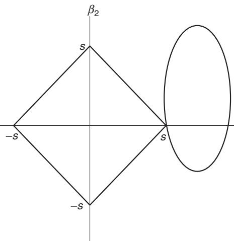
Figure 6.1: Model selection under Lasso.
Conversely, if , then and if then . These results can be summarized as follows:
Thus, for the coefficient estimate is set to 0. The larger is λ, the stronger the penalty and the more coefficients will be set to 0. See Tibshirani (1996) for further analysis and details.
We can also visualize the effect by considering the problem in two dimensions (i.e., only two covariates). To see this, consider the model
so we have a bivariate problem and can draw it in space. Assuming quadratic objectives, the objective function has contours that are ellipses in the space. Figure 6.1 visualizes this effect.
The LASSO constraints are now of the form , i.e.,
which creates a “diamond” around 0 with coordinates at , and . Figure 6.1 shows this graphically, where the diamond is the preceding set of constraints and the ellipse is drawn for that value of z that has the constraints binding. The chance that the ellipse intersects the constraints at a corner is high—as pictured in figure 6.1, we have at the constraint.
In practical applications a choice of λ must be made. Choosing delivers least squares estimates which means that the largest model almost always gets chosen. The larger the choice of , the more likely it is that individual are set to 0 and that a more parsimonious model is chosen. Unsurprisingly, the actual choice of or , since it is generally recommended to let it be a function of the sample size, T—impacts the properties of the method. Typical results provide rate conditions on rather than pinning down a specific value and are developed in fixed-regressor settings with i.i.d. data. For example, Belloni and Chernozhukov (2011) suggest setting for α near (but below) 1 and , where (·) is the normal c.d.f., and is the variance of the residuals from the true model.
The main difficulty in estimating the Lasso coefficients is that the objective function is nondifferentiable, so standard hill-climbing optimizers will not be useful for solving the minimization problem in (6.25). However, in recent years this estimation problem has been a subject of intense research and there now exist many methods that work well even when the dimension of X is very large.
Having selected a model by Lasso, a post-Lasso step can be added by estimating the parameter of the model using ordinary least squares or similar methods.
The Lasso approach has been extended to a wider group of penalized least squares estimators whose coefficients are estimated by minimizing
where is a penalty function. Bridge estimators set , where As a special case, if , Lasso is obtained, while yields the Ridge estimator. For this estimator retains the property that some of the estimates for will be 0 for large enough values of the penalties; see Fan and Li (2001) for theoretical results and Fan, Lv, and Qi (2011) for a review.
练习题
What is the primary purpose of the Lasso method in regression analysis?
Who introduced the Lasso method and in which year?
What effect does the tuning parameter have in the Lasso method?
What motivates the use of Lasso as a model selection tool? (Select all that apply)
In the Lasso approach, if , then must be 0.
The Lasso method always provides closed-form solutions for minimizing the objective function.
The Lasso coefficient estimate formula is given by . For , the coefficient estimate is set to ___.
Explain the effect of the tuning parameter in the Lasso method.
How does the Lasso method contribute to model selection in regression analysis?
Which of the following statements correctly describes the relationship between the Lasso tuning parameter and model selection?
Which of the following are true about the Lasso method and information criteria?
The Lasso method can be viewed as a special case of cross-validation for model selection.
In the Lasso method, the assumption that all variances of the predictors have been scaled to equal 1 ensures that the penalty term applies ___ to all predictors.
Explain how the Lasso method's tuning parameter influences the trade-off between model fit and model complexity.
登录后解锁笔记、知识点解析、AI 问答
立即登录